Metrics in QPyTorch

In this notebook, we will see how to evaluate QPyTorch models with probabilistic metrics.

Note: It is encouraged to check the Simple QP Regression notebook first if not done already. We’ll reuse most of the code from there.

We’ll be modeling the function

\[\begin{split}\begin{align} y &= \sin(2\pi x) + \epsilon \\ \epsilon &\sim \mathcal{N}(0, 0.04) \end{align}\end{split}\]

import math
import torch
import qpytorch
from matplotlib import pyplot as plt

%matplotlib inline
%load_ext autoreload
%autoreload 2

In the next cell, we set up the train and test data.

# Training data is 100 points in [0,1] inclusive regularly spaced
train_x = torch.linspace(0, 1, 100)
# True function is sin(2*pi*x) with Gaussian noise
train_y = torch.sin(train_x * (2 * math.pi)) + torch.randn(train_x.size()) * math.sqrt(0.04)

test_x = torch.linspace(0, 1, 51)
test_y = torch.sin(test_x * (2 * math.pi)) + torch.randn(test_x.size()) * math.sqrt(0.04)

In the next cell, we define a simple QP regression model.

# We will use the simplest form of QP model, exact inference
POWER = 1.0
class ExactQEPModel(qpytorch.models.ExactQEP):
    def __init__(self, train_x, train_y, likelihood):
        super(ExactQEPModel, self).__init__(train_x, train_y, likelihood)
        self.power = torch.tensor(POWER)
        self.mean_module = qpytorch.means.ConstantMean()
        self.covar_module = qpytorch.kernels.ScaleKernel(qpytorch.kernels.RBFKernel())

    def forward(self, x):
        mean_x = self.mean_module(x)
        covar_x = self.covar_module(x)
        return qpytorch.distributions.MultivariateQExponential(mean_x, covar_x, power=self.power)

# initialize likelihood and model
likelihood = qpytorch.likelihoods.QExponentialLikelihood(power=torch.tensor(POWER))
model = ExactQEPModel(train_x, train_y, likelihood)

Our model is ready for hyperparameter learning, but, first let us check how it performs on the test data.

model.eval()
with torch.no_grad():
    untrained_pred_dist = likelihood(model(test_x))
    predictive_mean = untrained_pred_dist.mean
    lower, upper = untrained_pred_dist.confidence_region()

f, ax = plt.subplots(1, 1, figsize=(4, 3))
# Plot training data as black stars
ax.plot(train_x, train_y, 'k*')
# Plot predictive means as blue line
ax.plot(test_x, predictive_mean, 'b')
# Shade between the lower and upper confidence bounds
ax.fill_between(test_x, lower, upper, alpha=0.5)
ax.set_ylim([-3, 3])
ax.legend(['Observed Data', 'Mean', 'Confidence'], bbox_to_anchor=(1.6,1));

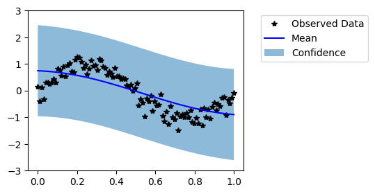
Visually, this does not look like a good fit. Now, let us train the model hyperparameters.

# this is for running the notebook in our testing framework
import os
smoke_test = ('CI' in os.environ)
training_iter = 2 if smoke_test else 80


# Find optimal model hyperparameters
model.train()

# Use the adam optimizer
optimizer = torch.optim.Adam(model.parameters(), lr=0.1)  # Includes QExponentialLikelihood parameters

# "Loss" for QEPs - the marginal log likelihood
mll = qpytorch.mlls.ExactMarginalLogLikelihood(likelihood, model)

for i in range(training_iter):
    # Zero gradients from previous iteration
    optimizer.zero_grad()
    # Output from model
    output = model(train_x)
    # Calc loss and backprop gradients
    loss = -mll(output, train_y)
    loss.backward()
    print('Iter %d/%d - Loss: %.3f   lengthscale: %.3f   noise: %.3f' % (
        i + 1, training_iter, loss.item(),
        model.covar_module.base_kernel.lengthscale.item(),
        model.likelihood.noise.item()
    ))
    optimizer.step()

Iter 1/80 - Loss: 1.700   lengthscale: 0.693   noise: 0.693
Iter 2/80 - Loss: 1.670   lengthscale: 0.644   noise: 0.644
Iter 3/80 - Loss: 1.636   lengthscale: 0.598   noise: 0.598
Iter 4/80 - Loss: 1.597   lengthscale: 0.555   noise: 0.554
Iter 5/80 - Loss: 1.551   lengthscale: 0.514   noise: 0.513
Iter 6/80 - Loss: 1.496   lengthscale: 0.475   noise: 0.474
Iter 7/80 - Loss: 1.434   lengthscale: 0.439   noise: 0.437
Iter 8/80 - Loss: 1.368   lengthscale: 0.405   noise: 0.402
Iter 9/80 - Loss: 1.304   lengthscale: 0.372   noise: 0.369
Iter 10/80 - Loss: 1.249   lengthscale: 0.342   noise: 0.339
Iter 11/80 - Loss: 1.204   lengthscale: 0.314   noise: 0.310
Iter 12/80 - Loss: 1.170   lengthscale: 0.289   noise: 0.284
Iter 13/80 - Loss: 1.143   lengthscale: 0.267   noise: 0.260
Iter 14/80 - Loss: 1.121   lengthscale: 0.248   noise: 0.237
Iter 15/80 - Loss: 1.101   lengthscale: 0.232   noise: 0.217
Iter 16/80 - Loss: 1.082   lengthscale: 0.219   noise: 0.198
Iter 17/80 - Loss: 1.065   lengthscale: 0.208   noise: 0.181
Iter 18/80 - Loss: 1.048   lengthscale: 0.199   noise: 0.165
Iter 19/80 - Loss: 1.032   lengthscale: 0.192   noise: 0.151
Iter 20/80 - Loss: 1.015   lengthscale: 0.186   noise: 0.138
Iter 21/80 - Loss: 0.998   lengthscale: 0.182   noise: 0.126
Iter 22/80 - Loss: 0.981   lengthscale: 0.180   noise: 0.115
Iter 23/80 - Loss: 0.963   lengthscale: 0.178   noise: 0.105
Iter 24/80 - Loss: 0.945   lengthscale: 0.177   noise: 0.096
Iter 25/80 - Loss: 0.926   lengthscale: 0.178   noise: 0.087
Iter 26/80 - Loss: 0.907   lengthscale: 0.179   noise: 0.080
Iter 27/80 - Loss: 0.888   lengthscale: 0.181   noise: 0.073
Iter 28/80 - Loss: 0.867   lengthscale: 0.184   noise: 0.066
Iter 29/80 - Loss: 0.847   lengthscale: 0.188   noise: 0.060
Iter 30/80 - Loss: 0.826   lengthscale: 0.193   noise: 0.055
Iter 31/80 - Loss: 0.805   lengthscale: 0.198   noise: 0.050
Iter 32/80 - Loss: 0.783   lengthscale: 0.205   noise: 0.046
Iter 33/80 - Loss: 0.761   lengthscale: 0.212   noise: 0.042
Iter 34/80 - Loss: 0.739   lengthscale: 0.220   noise: 0.038
Iter 35/80 - Loss: 0.717   lengthscale: 0.228   noise: 0.035
Iter 36/80 - Loss: 0.694   lengthscale: 0.238   noise: 0.032
Iter 37/80 - Loss: 0.672   lengthscale: 0.248   noise: 0.029
Iter 38/80 - Loss: 0.650   lengthscale: 0.259   noise: 0.026
Iter 39/80 - Loss: 0.627   lengthscale: 0.270   noise: 0.024
Iter 40/80 - Loss: 0.606   lengthscale: 0.283   noise: 0.022
Iter 41/80 - Loss: 0.584   lengthscale: 0.295   noise: 0.020
Iter 42/80 - Loss: 0.563   lengthscale: 0.309   noise: 0.018
Iter 43/80 - Loss: 0.542   lengthscale: 0.322   noise: 0.017
Iter 44/80 - Loss: 0.521   lengthscale: 0.336   noise: 0.015
Iter 45/80 - Loss: 0.501   lengthscale: 0.351   noise: 0.014
Iter 46/80 - Loss: 0.481   lengthscale: 0.365   noise: 0.013
Iter 47/80 - Loss: 0.462   lengthscale: 0.380   noise: 0.012
Iter 48/80 - Loss: 0.444   lengthscale: 0.394   noise: 0.011
Iter 49/80 - Loss: 0.426   lengthscale: 0.408   noise: 0.010
Iter 50/80 - Loss: 0.409   lengthscale: 0.421   noise: 0.009
Iter 51/80 - Loss: 0.393   lengthscale: 0.433   noise: 0.008
Iter 52/80 - Loss: 0.377   lengthscale: 0.444   noise: 0.007
Iter 53/80 - Loss: 0.362   lengthscale: 0.453   noise: 0.007
Iter 54/80 - Loss: 0.346   lengthscale: 0.461   noise: 0.006
Iter 55/80 - Loss: 0.331   lengthscale: 0.467   noise: 0.006
Iter 56/80 - Loss: 0.316   lengthscale: 0.471   noise: 0.005
Iter 57/80 - Loss: 0.302   lengthscale: 0.473   noise: 0.005
Iter 58/80 - Loss: 0.288   lengthscale: 0.474   noise: 0.004
Iter 59/80 - Loss: 0.274   lengthscale: 0.474   noise: 0.004
Iter 60/80 - Loss: 0.260   lengthscale: 0.473   noise: 0.004
Iter 61/80 - Loss: 0.247   lengthscale: 0.471   noise: 0.003
Iter 62/80 - Loss: 0.235   lengthscale: 0.468   noise: 0.003
Iter 63/80 - Loss: 0.224   lengthscale: 0.466   noise: 0.003
Iter 64/80 - Loss: 0.213   lengthscale: 0.463   noise: 0.003
Iter 65/80 - Loss: 0.202   lengthscale: 0.461   noise: 0.002
Iter 66/80 - Loss: 0.192   lengthscale: 0.458   noise: 0.002
Iter 67/80 - Loss: 0.183   lengthscale: 0.457   noise: 0.002
Iter 68/80 - Loss: 0.175   lengthscale: 0.456   noise: 0.002
Iter 69/80 - Loss: 0.166   lengthscale: 0.455   noise: 0.002
Iter 70/80 - Loss: 0.159   lengthscale: 0.455   noise: 0.002
Iter 71/80 - Loss: 0.151   lengthscale: 0.455   noise: 0.002
Iter 72/80 - Loss: 0.145   lengthscale: 0.456   noise: 0.001
Iter 73/80 - Loss: 0.138   lengthscale: 0.458   noise: 0.001
Iter 74/80 - Loss: 0.132   lengthscale: 0.460   noise: 0.001
Iter 75/80 - Loss: 0.127   lengthscale: 0.462   noise: 0.001
Iter 76/80 - Loss: 0.122   lengthscale: 0.464   noise: 0.001
Iter 77/80 - Loss: 0.117   lengthscale: 0.467   noise: 0.001
Iter 78/80 - Loss: 0.113   lengthscale: 0.469   noise: 0.001
Iter 79/80 - Loss: 0.109   lengthscale: 0.472   noise: 0.001
Iter 80/80 - Loss: 0.106   lengthscale: 0.474   noise: 0.001

In the next cell, we reevaluate the model on the test data.

model.eval()
with torch.no_grad():
    trained_pred_dist = likelihood(model(test_x))
    predictive_mean = trained_pred_dist.mean
    lower, upper = trained_pred_dist.confidence_region(rescale=True)

f, ax = plt.subplots(1, 1, figsize=(4, 3))
# Plot training data as black stars
ax.plot(train_x, train_y, 'k*')
# Plot predictive means as blue line
ax.plot(test_x, predictive_mean, 'b')
# Shade between the lower and upper confidence bounds
ax.fill_between(test_x, lower, upper, alpha=0.5)
ax.set_ylim([-3, 3])
ax.legend(['Observed Data', 'Mean', 'Confidence'], bbox_to_anchor=(1.6,1));

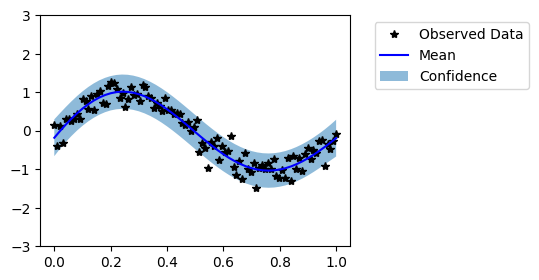
Now our model seems to fit well on the data. It is not always possible to visually evaluate the model in high dimensional cases. Thus, now we evaluate the models with help of probabilistic metrics. We have saved predictive distributions from untrained and trained models as untrained_pred_dist and trained_pred_dist respectively.

Negative Log Predictive Density (NLPD)

Negative Log Predictive Density (NLPD) is the most standard probabilistic metric for evaluating GP models. In simple terms, it is negative log likelihood of the test data given the predictive distribution. It can be computed as follows:

init_nlpd = qpytorch.metrics.negative_log_predictive_density(untrained_pred_dist, test_y)
final_nlpd = qpytorch.metrics.negative_log_predictive_density(trained_pred_dist, test_y)

print(f'Untrained model NLPD: {init_nlpd:.2f}, \nTrained model NLPD: {final_nlpd:.2f}')

Untrained model NLPD: 1.45,
Trained model NLPD: -0.29

Mean Standardized Log Loss (MSLL)

This metric computes average negative log likelihood of all test points w.r.t their univariate predicitve densities. For more details, see “page No. 23, Gaussian Processes for Machine Learning, Carl Edward Rasmussen and Christopher K. I. Williams, The MIT Press, 2006. ISBN 0-262-18253-X”

init_msll = qpytorch.metrics.mean_standardized_log_loss(untrained_pred_dist, test_y)
final_msll = qpytorch.metrics.mean_standardized_log_loss(trained_pred_dist, test_y)

print(f'Untrained model MSLL: {init_msll:.2f}, \nTrained model MSLL: {final_msll:.2f}')

Untrained model MSLL: 0.88,
Trained model MSLL: 13.94

It is also possible to calculate the quantile coverage error with qpytorch.metrics.quantile_coverage_error function.

quantile = 95
qce = qpytorch.metrics.quantile_coverage_error(trained_pred_dist, test_y, quantile=quantile)
print(f'Quantile {quantile}% Coverage Error: {qce:.2f}')

Quantile 95% Coverage Error: 0.56

Mean Squared Error (MSE)

Mean Squared Error (MSE) is the mean of the squared difference between the test observations and the predictive mean. It is a well-known conventional metric for evaluating regression models. However, it can not take uncertainty into account unlike NLPD, MLSS and ACE.

init_mse = qpytorch.metrics.mean_squared_error(untrained_pred_dist, test_y, squared=True)
final_mse = qpytorch.metrics.mean_squared_error(trained_pred_dist, test_y, squared=True)

print(f'Untrained model MSE: {init_mse:.2f}, \nTrained model MSE: {final_mse:.2f}')

Untrained model MSE: 0.19,
Trained model MSE: 0.03

Mean Absolute Error (MAE)

Mean Absolute Error (MAE) is the mean of the absolute difference between the test observations and the predictive mean. It is less sensitive to the outliers than MSE.

init_mae = qpytorch.metrics.mean_absolute_error(untrained_pred_dist, test_y)
final_mae = qpytorch.metrics.mean_absolute_error(trained_pred_dist, test_y)

print(f'Untrained model MAE: {init_mae:.2f}, \nTrained model MAE: {final_mae:.2f}')

Untrained model MAE: 0.37,
Trained model MAE: 0.13