QPyTorch Regression Tutorial
Introduction
In this notebook, we demonstrate many of the design features of QPyTorch using the simplest example, training an RBF kernel q-exponential process on a simple function. We’ll be modeling the function
with 100 training examples, and testing on 51 test examples.
Note: this notebook is not necessarily intended to teach the mathematical background of Gaussian/q-exponential processes, but rather how to train a simple one and make predictions in QPyTorch. For a mathematical treatment, Chapter 2 of Gaussian Processes for Machine Learning provides a very thorough introduction to GP regression (this entire text is highly recommended): http://www.gaussianprocess.org/gpml/chapters/RW2.pdf
[1]:
import math
import torch
import qpytorch
from matplotlib import pyplot as plt

%matplotlib inline
%load_ext autoreload
%autoreload 2
Set up training data
In the next cell, we set up the training data for this example. We’ll be using 100 regularly spaced points on [0,1] which we evaluate the function on and add Gaussian noise to get the training labels.
[2]:
# Training data is 100 points in [0,1] inclusive regularly spaced
train_x = torch.linspace(0, 1, 100)
# True function is sin(2*pi*x) with Gaussian noise
train_y = torch.sin(train_x * (2 * math.pi)) + torch.randn(train_x.size()) * math.sqrt(0.04)
Setting up the model
The next cell demonstrates the most critical features of a user-defined q-exponential process model in QPyTorch. Building a QEP model in QPyTorch is different in a number of ways.
First in contrast to many existing QEP packages, we do not provide full QEP models for the user. Rather, we provide the tools necessary to quickly construct one. This is because we believe, analogous to building a neural network in standard PyTorch, it is important to have the flexibility to include whatever components are necessary. As can be seen in more complicated examples, this allows the user great flexibility in designing custom models.
For most QEP regression models, you will need to construct the following QPyTorch objects:
A QEP Model (
qpytorch.models.ExactQEP) - This handles most of the inference.A Likelihood (
qpytorch.likelihoods.QExponentialLikelihood) - This is the most common likelihood used for QEP regression.A Mean - This defines the prior mean of the QEP.(If you don’t know which mean to use, a
qpytorch.means.ConstantMean()is a good place to start.)A Kernel - This defines the prior covariance of the QEP.(If you don’t know which kernel to use, a
qpytorch.kernels.ScaleKernel(qpytorch.kernels.RBFKernel())is a good place to start).A MultivariateQExponential Distribution (
qpytorch.distributions.MultivariateQExponential) - This is the object used to represent multivariate q-exponential distributions.
The QEP Model
The components of a user built (Exact, i.e. non-variational) QEP model in QPyTorch are, broadly speaking:
An
__init__method that takes the training data and a likelihood, and constructs whatever objects are necessary for the model’sforwardmethod. This will most commonly include things like a mean module and a kernel module.A
forwardmethod that takes in some \(n \times d\) dataxand returns aMultivariateQExponentialwith the prior mean and covariance evaluated atx. In other words, we return the vector \(\mu(x)\) and the \(n \times n\) matrix \(K_{xx}\) representing the prior mean and covariance matrix of the QEP.
This specification leaves a large amount of flexibility when defining a model. For example, to compose two kernels via addition, you can either add the kernel modules directly:
self.covar_module = ScaleKernel(RBFKernel() + LinearKernel())
Or you can add the outputs of the kernel in the forward method:
covar_x = self.rbf_kernel_module(x) + self.white_noise_module(x)
The likelihood
The simplest likelihood for regression is the qpytorch.likelihoods.QExponentialLikelihood. This assumes a homoskedastic noise model (i.e. all inputs have the same observational noise).
There are other options for exact QEP regression, such as the FixedNoiseQExponentialLikelihood, which assigns a different observed noise value to different training inputs.
[3]:
# We will use the simplest form of QEP model, exact inference
POWER = 1.0
class ExactQEPModel(qpytorch.models.ExactQEP):
    def __init__(self, train_x, train_y, likelihood):
        super(ExactQEPModel, self).__init__(train_x, train_y, likelihood)
        self.power = torch.tensor(POWER)
        self.mean_module = qpytorch.means.ConstantMean()
        self.covar_module = qpytorch.kernels.ScaleKernel(qpytorch.kernels.RBFKernel())

    def forward(self, x):
        mean_x = self.mean_module(x)
        covar_x = self.covar_module(x)
        return qpytorch.distributions.MultivariateQExponential(mean_x, covar_x, power=self.power)

# initialize likelihood and model
likelihood = qpytorch.likelihoods.QExponentialLikelihood(power=torch.tensor(POWER))
model = ExactQEPModel(train_x, train_y, likelihood)
Model modes
Like most PyTorch modules, the ExactQEP has a .train() and .eval() mode. - .train() mode is for optimizing model hyperameters. - .eval() mode is for computing predictions through the model posterior.
Training the model
In the next cell, we handle using Type-II MLE to train the hyperparameters of the q-exponential process.
The most obvious difference here compared to many other QEP implementations is that, as in standard PyTorch, the core training loop is written by the user. In QPyTorch, we make use of the standard PyTorch optimizers as from torch.optim, and all trainable parameters of the model should be of type torch.nn.Parameter. Because QEP models directly extend torch.nn.Module, calls to methods like model.parameters() or model.named_parameters() function as you might expect coming from
PyTorch.
In most cases, the boilerplate code below will work well. It has the same basic components as the standard PyTorch training loop:
Zero all parameter gradients
Call the model and compute the loss
Call backward on the loss to fill in gradients
Take a step on the optimizer
However, defining custom training loops allows for greater flexibility. For example, it is easy to save the parameters at each step of training, or use different learning rates for different parameters (which may be useful in deep kernel learning for example).
[4]:
# this is for running the notebook in our testing framework
import os
smoke_test = ('CI' in os.environ)
training_iter = 2 if smoke_test else 80


# Find optimal model hyperparameters
model.train()
likelihood.train()

# Use the adam optimizer
optimizer = torch.optim.Adam(model.parameters(), lr=0.1)  # Includes GaussianLikelihood parameters

# "Loss" for QEPs - the marginal log likelihood
mll = qpytorch.mlls.ExactMarginalLogLikelihood(likelihood, model)

for i in range(training_iter):
    # Zero gradients from previous iteration
    optimizer.zero_grad()
    # Output from model
    output = model(train_x)
    # Calc loss and backprop gradients
    loss = -mll(output, train_y)
    loss.backward()
    print('Iter %d/%d - Loss: %.3f   lengthscale: %.3f   noise: %.3f' % (
        i + 1, training_iter, loss.item(),
        model.covar_module.base_kernel.lengthscale.item(),
        model.likelihood.noise.item()
    ))
    optimizer.step()
Iter 1/80 - Loss: 1.678   lengthscale: 0.693   noise: 0.693
Iter 2/80 - Loss: 1.648   lengthscale: 0.644   noise: 0.644
Iter 3/80 - Loss: 1.614   lengthscale: 0.598   noise: 0.598
Iter 4/80 - Loss: 1.573   lengthscale: 0.555   noise: 0.554
Iter 5/80 - Loss: 1.524   lengthscale: 0.514   noise: 0.513
Iter 6/80 - Loss: 1.465   lengthscale: 0.476   noise: 0.474
Iter 7/80 - Loss: 1.396   lengthscale: 0.440   noise: 0.437
Iter 8/80 - Loss: 1.321   lengthscale: 0.406   noise: 0.402
Iter 9/80 - Loss: 1.246   lengthscale: 0.373   noise: 0.369
Iter 10/80 - Loss: 1.178   lengthscale: 0.343   noise: 0.338
Iter 11/80 - Loss: 1.122   lengthscale: 0.315   noise: 0.310
Iter 12/80 - Loss: 1.079   lengthscale: 0.289   noise: 0.284
Iter 13/80 - Loss: 1.045   lengthscale: 0.266   noise: 0.259
Iter 14/80 - Loss: 1.017   lengthscale: 0.247   noise: 0.237
Iter 15/80 - Loss: 0.991   lengthscale: 0.230   noise: 0.216
Iter 16/80 - Loss: 0.969   lengthscale: 0.215   noise: 0.197
Iter 17/80 - Loss: 0.949   lengthscale: 0.203   noise: 0.180
Iter 18/80 - Loss: 0.930   lengthscale: 0.192   noise: 0.164
Iter 19/80 - Loss: 0.913   lengthscale: 0.183   noise: 0.150
Iter 20/80 - Loss: 0.895   lengthscale: 0.176   noise: 0.137
Iter 21/80 - Loss: 0.879   lengthscale: 0.171   noise: 0.125
Iter 22/80 - Loss: 0.862   lengthscale: 0.166   noise: 0.114
Iter 23/80 - Loss: 0.845   lengthscale: 0.163   noise: 0.104
Iter 24/80 - Loss: 0.827   lengthscale: 0.161   noise: 0.095
Iter 25/80 - Loss: 0.810   lengthscale: 0.159   noise: 0.087
Iter 26/80 - Loss: 0.792   lengthscale: 0.159   noise: 0.079
Iter 27/80 - Loss: 0.773   lengthscale: 0.159   noise: 0.072
Iter 28/80 - Loss: 0.754   lengthscale: 0.160   noise: 0.066
Iter 29/80 - Loss: 0.735   lengthscale: 0.162   noise: 0.060
Iter 30/80 - Loss: 0.715   lengthscale: 0.165   noise: 0.055
Iter 31/80 - Loss: 0.694   lengthscale: 0.168   noise: 0.050
Iter 32/80 - Loss: 0.674   lengthscale: 0.172   noise: 0.046
Iter 33/80 - Loss: 0.653   lengthscale: 0.177   noise: 0.042
Iter 34/80 - Loss: 0.631   lengthscale: 0.182   noise: 0.038
Iter 35/80 - Loss: 0.610   lengthscale: 0.188   noise: 0.035
Iter 36/80 - Loss: 0.588   lengthscale: 0.194   noise: 0.032
Iter 37/80 - Loss: 0.566   lengthscale: 0.201   noise: 0.029
Iter 38/80 - Loss: 0.544   lengthscale: 0.209   noise: 0.027
Iter 39/80 - Loss: 0.522   lengthscale: 0.217   noise: 0.024
Iter 40/80 - Loss: 0.500   lengthscale: 0.226   noise: 0.022
Iter 41/80 - Loss: 0.479   lengthscale: 0.236   noise: 0.020
Iter 42/80 - Loss: 0.457   lengthscale: 0.245   noise: 0.019
Iter 43/80 - Loss: 0.436   lengthscale: 0.256   noise: 0.017
Iter 44/80 - Loss: 0.414   lengthscale: 0.267   noise: 0.016
Iter 45/80 - Loss: 0.393   lengthscale: 0.278   noise: 0.014
Iter 46/80 - Loss: 0.373   lengthscale: 0.289   noise: 0.013
Iter 47/80 - Loss: 0.352   lengthscale: 0.301   noise: 0.012
Iter 48/80 - Loss: 0.332   lengthscale: 0.313   noise: 0.011
Iter 49/80 - Loss: 0.312   lengthscale: 0.326   noise: 0.010
Iter 50/80 - Loss: 0.293   lengthscale: 0.338   noise: 0.009
Iter 51/80 - Loss: 0.273   lengthscale: 0.351   noise: 0.008
Iter 52/80 - Loss: 0.254   lengthscale: 0.364   noise: 0.008
Iter 53/80 - Loss: 0.236   lengthscale: 0.377   noise: 0.007
Iter 54/80 - Loss: 0.217   lengthscale: 0.390   noise: 0.006
Iter 55/80 - Loss: 0.200   lengthscale: 0.404   noise: 0.006
Iter 56/80 - Loss: 0.183   lengthscale: 0.416   noise: 0.005
Iter 57/80 - Loss: 0.167   lengthscale: 0.429   noise: 0.005
Iter 58/80 - Loss: 0.151   lengthscale: 0.440   noise: 0.004
Iter 59/80 - Loss: 0.136   lengthscale: 0.451   noise: 0.004
Iter 60/80 - Loss: 0.121   lengthscale: 0.461   noise: 0.004
Iter 61/80 - Loss: 0.107   lengthscale: 0.469   noise: 0.003
Iter 62/80 - Loss: 0.093   lengthscale: 0.476   noise: 0.003
Iter 63/80 - Loss: 0.079   lengthscale: 0.482   noise: 0.003
Iter 64/80 - Loss: 0.066   lengthscale: 0.486   noise: 0.003
Iter 65/80 - Loss: 0.053   lengthscale: 0.488   noise: 0.002
Iter 66/80 - Loss: 0.040   lengthscale: 0.490   noise: 0.002
Iter 67/80 - Loss: 0.028   lengthscale: 0.490   noise: 0.002
Iter 68/80 - Loss: 0.017   lengthscale: 0.489   noise: 0.002
Iter 69/80 - Loss: 0.005   lengthscale: 0.488   noise: 0.002
Iter 70/80 - Loss: -0.005   lengthscale: 0.487   noise: 0.002
Iter 71/80 - Loss: -0.015   lengthscale: 0.485   noise: 0.002
Iter 72/80 - Loss: -0.025   lengthscale: 0.483   noise: 0.001
Iter 73/80 - Loss: -0.033   lengthscale: 0.481   noise: 0.001
Iter 74/80 - Loss: -0.042   lengthscale: 0.479   noise: 0.001
Iter 75/80 - Loss: -0.049   lengthscale: 0.478   noise: 0.001
Iter 76/80 - Loss: -0.057   lengthscale: 0.477   noise: 0.001
Iter 77/80 - Loss: -0.063   lengthscale: 0.477   noise: 0.001
Iter 78/80 - Loss: -0.070   lengthscale: 0.477   noise: 0.001
Iter 79/80 - Loss: -0.076   lengthscale: 0.477   noise: 0.001
Iter 80/80 - Loss: -0.081   lengthscale: 0.478   noise: 0.001
Make predictions with the model
In the next cell, we make predictions with the model. To do this, we simply put the model and likelihood in eval mode, and call both modules on the test data.
Just as a user defined QEP model returns a MultivariateQExponential containing the prior mean and covariance from forward, a trained QEP model in eval mode returns a MultivariateQExponential containing the posterior mean and covariance.
If we denote a test point (test_x) as x* with the true output being y*, then model(test_x) returns the model posterior distribution p(f* | x*, X, y), for training data X, y. This posterior is the distribution over the function we are trying to model, and thus quantifies our model uncertainty.
In contrast, likelihood(model(test_x)) gives us the posterior predictive distribution p(y* | x*, X, y) which is the probability distribution over the predicted output value. Recall in our problem setup
where 𝜖 is the likelihood noise for each observation. By including the likelihood noise which is the noise in your observation (e.g. due to noisy sensor), the prediction is over the observed value of the test point.
Thus, getting the predictive mean and variance, and then sampling functions from the QEP at the given test points could be accomplished with calls like:
f_preds = model(test_x)
y_preds = likelihood(model(test_x))

f_mean = f_preds.mean
f_var = f_preds.variance
f_covar = f_preds.covariance_matrix
f_samples = f_preds.sample(sample_shape=torch.Size(1000,))
The qpytorch.settings.fast_pred_var context is not needed, but here we are giving a preview of using one of our cool features, getting faster predictive distributions using LOVE.
[5]:
# Get into evaluation (predictive posterior) mode
model.eval()
likelihood.eval()

# Test points are regularly spaced along [0,1]
# Make predictions by feeding model through likelihood
with torch.no_grad(), qpytorch.settings.fast_pred_var():
    test_x = torch.linspace(0, 1, 51)
    observed_pred = likelihood(model(test_x))
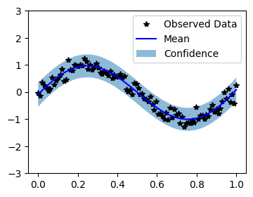
Plot the model fit
In the next cell, we plot the mean and confidence region of the Gaussian process model. The confidence_region method is a helper method that returns 2 standard deviations above and below the mean.
[6]:
with torch.no_grad():
    # Initialize plot
    f, ax = plt.subplots(1, 1, figsize=(4, 3))

    # Get upper and lower confidence bounds
    lower, upper = observed_pred.confidence_region(rescale=True)
    # Plot training data as black stars
    ax.plot(train_x.numpy(), train_y.numpy(), 'k*')
    # Plot predictive means as blue line
    ax.plot(test_x.numpy(), observed_pred.mean.numpy(), 'b')
    # Shade between the lower and upper confidence bounds
    ax.fill_between(test_x.numpy(), lower.numpy(), upper.numpy(), alpha=0.5)
    ax.set_ylim([-3, 3])
    ax.legend(['Observed Data', 'Mean', 'Confidence'])