Variational QEP with derivative information in 2d
Introduction
In this example, we show how to train an approximate/variational QEP model in QPyTorch of a 2-dimensional function given function values and derivative observations. We consider modeling the Franke functions where the values and derivatives are contaminated with independent \(\mathcal{N}(0, 0.05^2)\) distributed noise.
[1]:
import torch
import qpytorch
import math
from matplotlib import cm
from matplotlib import pyplot as plt
import numpy as np

%matplotlib inline
%load_ext autoreload
%autoreload 2
Franke function
The following is a vectorized implementation of the 2-dimensional Franke function ((https://www.sfu.ca/~ssurjano/franke2d.html)). To make it more challenging than GPyTorch implementation, we include the second order derivatives.
[2]:
# generate data
def franke(X, Y):
    term1 = .75*torch.exp(-((9*X - 2).pow(2) + (9*Y - 2).pow(2))/4)
    term2 = .75*torch.exp(-((9*X + 1).pow(2))/49 - (9*Y + 1)/10)
    term3 = .5*torch.exp(-((9*X - 7).pow(2) + (9*Y - 3).pow(2))/4)
    term4 = .2*torch.exp(-(9*X - 4).pow(2) - (9*Y - 7).pow(2))

    f = term1 + term2 + term3 - term4
    dfx = -2*(9*X - 2)*9/4 * term1 - 2*(9*X + 1)*9/49 * term2 + \
          -2*(9*X - 7)*9/4 * term3 + 2*(9*X - 4)*9 * term4
    dfy = -2*(9*Y - 2)*9/4 * term1 - 9/10 * term2 + \
          -2*(9*Y - 3)*9/4 * term3 + 2*(9*Y - 7)*9 * term4
    d2fx = ((2*(9*X - 2)*9/4)**2 - 2*9*9/4) * term1 + ((2*(9*X + 1)*9/49)**2 - 2*9*9/49) * term2 + \
          +((2*(9*X - 7)*9/4)**2 - 2*9*9/4) * term3 - ((2*(9*X - 4)*9)**2 - 2*9*9) * term4
    d2fy = ((2*(9*Y - 2)*9/4)**2 - 2*9*9/4) * term1 + (9/10)**2 * term2 + \
          +((2*(9*Y - 3)*9/4)**2 - 2*9*9/4) * term3 - ((2*(9*Y - 7)*9)**2 - 2*9*9) * term4

    return f, dfx, dfy, d2fx, d2fy
Setting up the training data
We use a grid with 225 points in \([0,1] \times [0,1]\) with 15 uniformly distributed points per dimension.
[3]:
xv, yv = torch.meshgrid(torch.linspace(0, 1, 15), torch.linspace(0, 1, 15), indexing="ij")
train_x = torch.cat((
    xv.contiguous().view(xv.numel(), 1),
    yv.contiguous().view(yv.numel(), 1)),
    dim=1
)

f, dfx, dfy, d2fx, d2fy = franke(train_x[:, 0], train_x[:, 1])
train_y = torch.stack([f, dfx, dfy, d2fx, d2fy], -1).squeeze(1)

train_y += 0.05 * torch.randn(train_y.size()) # Add noise to both values and gradients
lb, ub = 0, 1.0
Setting up the model
A QEP prior on the function values implies a multi-output QEP prior on the function values and the partial derivatives, see 9.4 in http://www.gaussianprocess.org/gpml/chapters/RW9.pdf for more details. This allows using a MultitaskMultivariateQExponential and MultitaskQExponentialLikelihood to train an exact QEP model from both function values and gradients.
However, if we want to use variational QEP, the standard VariationalStrategy does not take multitask variational distribution. To overcome this issue, QPyTorch extends VariationalStrategy to MultitaskVariationalStrategy so that it works with MultitaskMultivariateQExponential. The resulting Matern52 kernel that models the covariance between the values and partial derivatives has been implemented in Matern52KernelGradGrad to include upto second order derivatives and the
extension of a linear mean is implemented in LinearMeanGradGrad.
[4]:
POWER = 1.0
class QEPModelWithDerivatives(qpytorch.models.ApproximateQEP):
    def __init__(self, input_dims, output_dims, num_inducing=128, likelihood=None):
        self.power = torch.tensor(POWER)
        inducing_points = lb + torch.rand(output_dims,num_inducing, input_dims) * (ub-lb)
        # inducing_points = train_x[torch.randperm(train_x.size(0))[:num_inducing]]
        batch_shape = torch.Size([output_dims])
        variational_distribution = qpytorch.variational.CholeskyVariationalDistribution(
            num_inducing_points=num_inducing,
            batch_shape=batch_shape,
            power=self.power
        )
        variational_strategy = qpytorch.variational.MultitaskVariationalStrategy(
            self,
            inducing_points,
            variational_distribution,
            learn_inducing_locations=True,
            # jitter_val = 1.0e-4
        )

        super().__init__(variational_strategy)
        self.mean_module = qpytorch.means.LinearMeanGradGrad(input_dims)
        self.base_kernel = qpytorch.kernels.Matern52KernelGradGrad(ard_num_dims=input_dims, eps=1e-4, interleaved=False)
        self.covar_module = qpytorch.kernels.ScaleKernel(self.base_kernel)
        self.covar_module.base_kernel.register_constraint("raw_lengthscale", qpytorch.constraints.Interval(1e-2, 2))
        self.likelihood = likelihood

    def forward(self, x):
        mean_x = self.mean_module(x) # ... x N x (D+1)
        covar_x = self.covar_module(x) # ... x N(D+1) x N(D+1)
        return qpytorch.distributions.MultitaskMultivariateQExponential(mean_x, covar_x, power=POWER, interleaved=False)

likelihood = qpytorch.likelihoods.MultitaskQExponentialLikelihood(num_tasks=train_y.size(-1), power=torch.tensor(POWER),
                                                                  noise_constraint=qpytorch.constraints.Interval(1e-2,2))  # Value + Derivative
model = QEPModelWithDerivatives(train_x.size(-1), train_y.size(-1), likelihood=likelihood)
The model training is similar to training a standard variational QEP regression model.
[5]:
# this is for running the notebook in our testing framework
import os
smoke_test = ('CI' in os.environ)
training_iter = 2 if smoke_test else 50


# Find optimal model hyperparameters
model.train()

# Use the adam optimizer
optimizer = torch.optim.Adam(model.parameters(), lr=0.05)  # Includes QExponentialLikelihood parameters

# "Loss" for QEPs - the marginal log likelihood
mll = qpytorch.mlls.VariationalELBO(likelihood, model, num_data=train_y.size(0))

for i in range(training_iter):
    optimizer.zero_grad()
    output = model(train_x)
    loss = -mll(output, train_y).sum()
    loss.backward()
    print("Iter %d/%d - Loss: %.3f   lengthscales: %.3f, %.3f   noise: %.3f" % (
        i + 1, training_iter, loss.item(),
        model.covar_module.base_kernel.lengthscale.squeeze()[0],
        model.covar_module.base_kernel.lengthscale.squeeze()[1],
        model.likelihood.noise.item()
    ))
    optimizer.step()
Iter 1/50 - Loss: 92.150   lengthscales: 1.005, 1.005   noise: 1.005
Iter 2/50 - Loss: 89.432   lengthscales: 1.030, 1.030   noise: 1.030
Iter 3/50 - Loss: 86.067   lengthscales: 1.055, 1.055   noise: 1.055
Iter 4/50 - Loss: 83.225   lengthscales: 1.079, 1.079   noise: 1.079
Iter 5/50 - Loss: 80.565   lengthscales: 1.103, 1.102   noise: 1.103
Iter 6/50 - Loss: 78.135   lengthscales: 1.126, 1.125   noise: 1.126
Iter 7/50 - Loss: 75.887   lengthscales: 1.149, 1.147   noise: 1.149
Iter 8/50 - Loss: 73.703   lengthscales: 1.170, 1.167   noise: 1.171
Iter 9/50 - Loss: 71.835   lengthscales: 1.191, 1.187   noise: 1.193
Iter 10/50 - Loss: 69.881   lengthscales: 1.211, 1.204   noise: 1.213
Iter 11/50 - Loss: 68.241   lengthscales: 1.230, 1.220   noise: 1.233
Iter 12/50 - Loss: 66.479   lengthscales: 1.247, 1.235   noise: 1.252
Iter 13/50 - Loss: 64.905   lengthscales: 1.264, 1.247   noise: 1.269
Iter 14/50 - Loss: 63.350   lengthscales: 1.279, 1.258   noise: 1.286
Iter 15/50 - Loss: 61.875   lengthscales: 1.293, 1.267   noise: 1.302
Iter 16/50 - Loss: 60.524   lengthscales: 1.306, 1.275   noise: 1.317
Iter 17/50 - Loss: 59.266   lengthscales: 1.318, 1.281   noise: 1.330
Iter 18/50 - Loss: 58.156   lengthscales: 1.328, 1.286   noise: 1.343
Iter 19/50 - Loss: 57.286   lengthscales: 1.338, 1.290   noise: 1.355
Iter 20/50 - Loss: 56.247   lengthscales: 1.347, 1.292   noise: 1.366
Iter 21/50 - Loss: 55.404   lengthscales: 1.354, 1.293   noise: 1.377
Iter 22/50 - Loss: 54.651   lengthscales: 1.361, 1.293   noise: 1.386
Iter 23/50 - Loss: 53.703   lengthscales: 1.367, 1.291   noise: 1.395
Iter 24/50 - Loss: 52.957   lengthscales: 1.373, 1.288   noise: 1.402
Iter 25/50 - Loss: 52.314   lengthscales: 1.377, 1.284   noise: 1.409
Iter 26/50 - Loss: 51.711   lengthscales: 1.381, 1.278   noise: 1.416
Iter 27/50 - Loss: 50.835   lengthscales: 1.384, 1.271   noise: 1.421
Iter 28/50 - Loss: 50.541   lengthscales: 1.386, 1.263   noise: 1.426
Iter 29/50 - Loss: 49.773   lengthscales: 1.386, 1.254   noise: 1.430
Iter 30/50 - Loss: 49.010   lengthscales: 1.386, 1.245   noise: 1.433
Iter 31/50 - Loss: 48.403   lengthscales: 1.385, 1.235   noise: 1.436
Iter 32/50 - Loss: 47.581   lengthscales: 1.383, 1.225   noise: 1.438
Iter 33/50 - Loss: 47.059   lengthscales: 1.379, 1.215   noise: 1.439
Iter 34/50 - Loss: 46.518   lengthscales: 1.375, 1.205   noise: 1.440
Iter 35/50 - Loss: 45.828   lengthscales: 1.369, 1.194   noise: 1.440
Iter 36/50 - Loss: 45.416   lengthscales: 1.362, 1.184   noise: 1.439
Iter 37/50 - Loss: 44.877   lengthscales: 1.354, 1.175   noise: 1.438
Iter 38/50 - Loss: 44.311   lengthscales: 1.344, 1.166   noise: 1.435
Iter 39/50 - Loss: 43.798   lengthscales: 1.333, 1.159   noise: 1.433
Iter 40/50 - Loss: 43.406   lengthscales: 1.321, 1.153   noise: 1.429
Iter 41/50 - Loss: 43.045   lengthscales: 1.308, 1.147   noise: 1.425
Iter 42/50 - Loss: 42.490   lengthscales: 1.293, 1.142   noise: 1.419
Iter 43/50 - Loss: 42.428   lengthscales: 1.276, 1.140   noise: 1.414
Iter 44/50 - Loss: 41.433   lengthscales: 1.259, 1.138   noise: 1.407
Iter 45/50 - Loss: 40.827   lengthscales: 1.241, 1.137   noise: 1.399
Iter 46/50 - Loss: 40.518   lengthscales: 1.222, 1.136   noise: 1.391
Iter 47/50 - Loss: 40.044   lengthscales: 1.203, 1.136   noise: 1.382
Iter 48/50 - Loss: 39.340   lengthscales: 1.183, 1.135   noise: 1.371
Iter 49/50 - Loss: 38.700   lengthscales: 1.164, 1.133   noise: 1.360
Iter 50/50 - Loss: 38.742   lengthscales: 1.145, 1.131   noise: 1.348
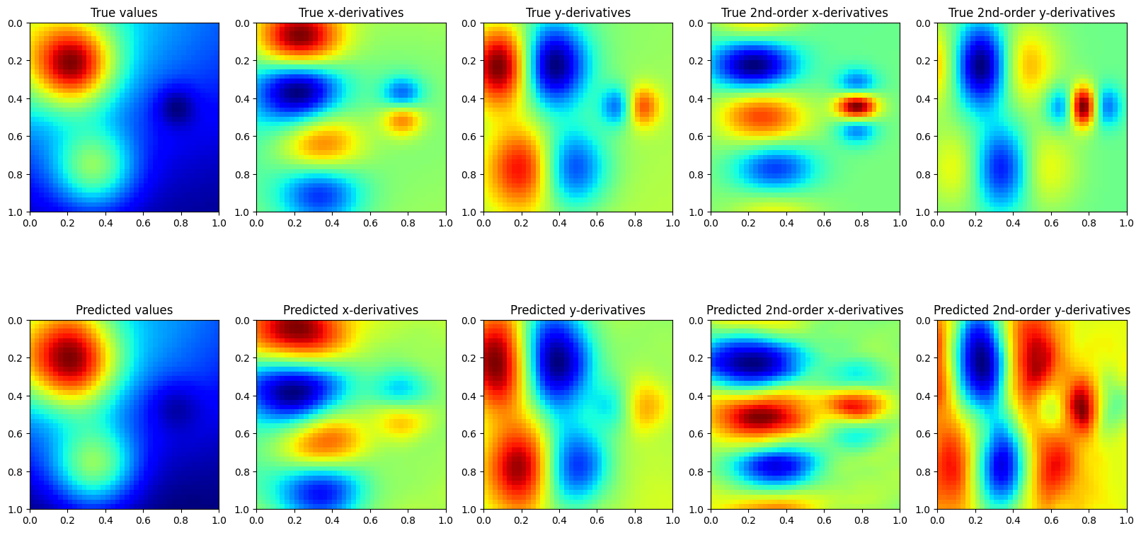
Model predictions are also similar to QEP regression with only function values, but we need more CG iterations to get accurate estimates of the predictive variance
[6]:
# Set into eval mode
model.eval()

# Initialize plots
fig, ax = plt.subplots(2, train_y.size(-1), figsize=(20, 10))

# Test points
n1, n2 = 40, 40
xv, yv = torch.meshgrid(torch.linspace(0, 1, n1), torch.linspace(0, 1, n2), indexing="ij")
f, dfx, dfy, d2fx, d2fy = franke(xv, yv)

# Make predictions
with torch.no_grad(), qpytorch.settings.fast_computations(log_prob=False, covar_root_decomposition=False):
    test_x = torch.stack([xv.reshape(n1*n2, 1), yv.reshape(n1*n2, 1)], -1).squeeze(1)
    predictions = likelihood(model(test_x))
    mean = predictions.mean
    if mean.ndim == 3: mean = mean.mean(0)

extent = (xv.min(), xv.max(), yv.max(), yv.min())
ax[0, 0].imshow(f, extent=extent, cmap=cm.jet)
ax[0, 0].set_title('True values')
ax[0, 1].imshow(dfx, extent=extent, cmap=cm.jet)
ax[0, 1].set_title('True x-derivatives')
ax[0, 2].imshow(dfy, extent=extent, cmap=cm.jet)
ax[0, 2].set_title('True y-derivatives')
ax[0, 3].imshow(d2fx, extent=extent, cmap=cm.jet)
ax[0, 3].set_title('True 2nd-order x-derivatives')
ax[0, 4].imshow(d2fy, extent=extent, cmap=cm.jet)
ax[0, 4].set_title('True 2nd-order y-derivatives')

ax[1, 0].imshow(mean[:, 0].detach().numpy().reshape(n1, n2), extent=extent, cmap=cm.jet)
ax[1, 0].set_title('Predicted values')
ax[1, 1].imshow(mean[:, 1].detach().numpy().reshape(n1, n2), extent=extent, cmap=cm.jet)
ax[1, 1].set_title('Predicted x-derivatives')
ax[1, 2].imshow(mean[:, 2].detach().numpy().reshape(n1, n2), extent=extent, cmap=cm.jet)
ax[1, 2].set_title('Predicted y-derivatives')
ax[1, 3].imshow(mean[:, 3].detach().numpy().reshape(n1, n2), extent=extent, cmap=cm.jet)
ax[1, 3].set_title('Predicted 2nd-order x-derivatives')
ax[1, 4].imshow(mean[:, 4].detach().numpy().reshape(n1, n2), extent=extent, cmap=cm.jet)
ax[1, 4].set_title('Predicted 2nd-order y-derivatives')

None