QEP Regression with Grid Structured Training Data

In this notebook, we demonstrate how to perform QEP regression when your training data lies on a regularly spaced grid. For this example, we’ll be modeling a 2D function where the training data is on an evenly spaced grid on (0,1)x(0, 2) with 100 grid points in each dimension.

In other words, we have 10000 training examples. However, the grid structure of the training data will allow us to perform inference very quickly anyways.

import qpytorch
import torch
import math

Make the grid and training data

In the next cell, we create the grid, along with the 10000 training examples and labels. After running this cell, we create three important tensors:

• grid is a tensor that is grid_size x 2 and contains the 1D grid for each dimension.

• train_x is a tensor containing the full 10000 training examples.

• train_y are the labels. For this, we’re just using a simple sine function.

grid_bounds = [(0, 1), (0, 2)]
grid_size = 25
grid = torch.zeros(grid_size, len(grid_bounds))
for i in range(len(grid_bounds)):
    grid_diff = float(grid_bounds[i][1] - grid_bounds[i][0]) / (grid_size - 2)
    grid[:, i] = torch.linspace(grid_bounds[i][0] - grid_diff, grid_bounds[i][1] + grid_diff, grid_size)

train_x = qpytorch.utils.grid.create_data_from_grid(grid)
train_y = torch.sin((train_x[:, 0] + train_x[:, 1]) * (2 * math.pi)) + torch.randn_like(train_x[:, 0]).mul(0.01)

Creating the Grid QEP Model

In the next cell we create our QEP model. Like other scalable QEP methods, we’ll use a scalable kernel that wraps a base kernel. In this case, we create a GridKernel that wraps an RBFKernel.

POWER = 1.0
class GridQEPRegressionModel(qpytorch.models.ExactQEP):
    def __init__(self, grid, train_x, train_y, likelihood):
        super(GridQEPRegressionModel, self).__init__(train_x, train_y, likelihood)
        self.power = torch.tensor(POWER)
        num_dims = train_x.size(-1)
        self.mean_module = qpytorch.means.ConstantMean()
        self.covar_module = qpytorch.kernels.GridKernel(qpytorch.kernels.RBFKernel(), grid=grid)

    def forward(self, x):
        mean_x = self.mean_module(x)
        covar_x = self.covar_module(x)
        return qpytorch.distributions.MultivariateQExponential(mean_x, covar_x, power=self.power)

likelihood = qpytorch.likelihoods.QExponentialLikelihood(power=torch.tensor(POWER))
model = GridQEPRegressionModel(grid, train_x, train_y, likelihood)

# this is for running the notebook in our testing framework
import os
smoke_test = ('CI' in os.environ)
training_iter = 2 if smoke_test else 50


# Find optimal model hyperparameters
model.train()
likelihood.train()

# Use the adam optimizer
optimizer = torch.optim.Adam(model.parameters(), lr=0.1)  # Includes QExponentialLikelihood parameters

# "Loss" for QEPs - the marginal log likelihood
mll = qpytorch.mlls.ExactMarginalLogLikelihood(likelihood, model)

for i in range(training_iter):
    # Zero gradients from previous iteration
    optimizer.zero_grad()
    # Output from model
    output = model(train_x)
    # Calc loss and backprop gradients
    loss = -mll(output, train_y)
    loss.backward()
    print('Iter %d/%d - Loss: %.3f   lengthscale: %.3f   noise: %.3f' % (
        i + 1, training_iter, loss.item(),
        model.covar_module.base_kernel.lengthscale.item(),
        model.likelihood.noise.item()
    ))
    optimizer.step()

Iter 1/50 - Loss: 2.289   lengthscale: 0.693   noise: 0.693
Iter 2/50 - Loss: 2.266   lengthscale: 0.644   noise: 0.644
Iter 3/50 - Loss: 2.240   lengthscale: 0.599   noise: 0.598
Iter 4/50 - Loss: 2.209   lengthscale: 0.556   noise: 0.554
Iter 5/50 - Loss: 2.171   lengthscale: 0.517   noise: 0.513
Iter 6/50 - Loss: 2.124   lengthscale: 0.480   noise: 0.474
Iter 7/50 - Loss: 2.062   lengthscale: 0.446   noise: 0.437
Iter 8/50 - Loss: 1.983   lengthscale: 0.414   noise: 0.402
Iter 9/50 - Loss: 1.888   lengthscale: 0.383   noise: 0.369
Iter 10/50 - Loss: 1.778   lengthscale: 0.354   noise: 0.338
Iter 11/50 - Loss: 1.658   lengthscale: 0.326   noise: 0.310
Iter 12/50 - Loss: 1.538   lengthscale: 0.300   noise: 0.283
Iter 13/50 - Loss: 1.425   lengthscale: 0.274   noise: 0.258
Iter 14/50 - Loss: 1.327   lengthscale: 0.251   noise: 0.235
Iter 15/50 - Loss: 1.244   lengthscale: 0.229   noise: 0.213
Iter 16/50 - Loss: 1.176   lengthscale: 0.210   noise: 0.193
Iter 17/50 - Loss: 1.122   lengthscale: 0.193   noise: 0.175
Iter 18/50 - Loss: 1.081   lengthscale: 0.178   noise: 0.158
Iter 19/50 - Loss: 1.047   lengthscale: 0.166   noise: 0.143
Iter 20/50 - Loss: 1.019   lengthscale: 0.157   noise: 0.129
Iter 21/50 - Loss: 0.994   lengthscale: 0.149   noise: 0.117
Iter 22/50 - Loss: 0.968   lengthscale: 0.143   noise: 0.105
Iter 23/50 - Loss: 0.939   lengthscale: 0.140   noise: 0.095
Iter 24/50 - Loss: 0.907   lengthscale: 0.138   noise: 0.086
Iter 25/50 - Loss: 0.869   lengthscale: 0.138   noise: 0.077
Iter 26/50 - Loss: 0.827   lengthscale: 0.139   noise: 0.070
Iter 27/50 - Loss: 0.779   lengthscale: 0.141   noise: 0.063
Iter 28/50 - Loss: 0.728   lengthscale: 0.145   noise: 0.056
Iter 29/50 - Loss: 0.675   lengthscale: 0.150   noise: 0.051
Iter 30/50 - Loss: 0.619   lengthscale: 0.155   noise: 0.046
Iter 31/50 - Loss: 0.563   lengthscale: 0.162   noise: 0.041
Iter 32/50 - Loss: 0.508   lengthscale: 0.169   noise: 0.037
Iter 33/50 - Loss: 0.454   lengthscale: 0.177   noise: 0.033
Iter 34/50 - Loss: 0.403   lengthscale: 0.186   noise: 0.030
Iter 35/50 - Loss: 0.355   lengthscale: 0.194   noise: 0.027
Iter 36/50 - Loss: 0.310   lengthscale: 0.203   noise: 0.024
Iter 37/50 - Loss: 0.267   lengthscale: 0.211   noise: 0.022
Iter 38/50 - Loss: 0.226   lengthscale: 0.219   noise: 0.020
Iter 39/50 - Loss: 0.186   lengthscale: 0.226   noise: 0.018
Iter 40/50 - Loss: 0.147   lengthscale: 0.231   noise: 0.016
Iter 41/50 - Loss: 0.107   lengthscale: 0.235   noise: 0.014
Iter 42/50 - Loss: 0.065   lengthscale: 0.238   noise: 0.013
Iter 43/50 - Loss: 0.023   lengthscale: 0.239   noise: 0.011
Iter 44/50 - Loss: -0.021   lengthscale: 0.239   noise: 0.010
Iter 45/50 - Loss: -0.066   lengthscale: 0.238   noise: 0.009
Iter 46/50 - Loss: -0.110   lengthscale: 0.236   noise: 0.008
Iter 47/50 - Loss: -0.154   lengthscale: 0.233   noise: 0.007
Iter 48/50 - Loss: -0.197   lengthscale: 0.230   noise: 0.007
Iter 49/50 - Loss: -0.239   lengthscale: 0.227   noise: 0.006
Iter 50/50 - Loss: -0.279   lengthscale: 0.224   noise: 0.005

In the next cell, we create a set of 400 test examples and make predictions. Note that unlike other scalable QEP methods, testing is more complicated. Because our test data can be different from the training data, in general we may not be able to avoid creating a num_train x num_test (e.g., 10000 x 400) kernel matrix between the training and test data.

For this reason, if you have large numbers of test points, memory may become a concern. The time complexity should still be reasonable, however, because we will still exploit structure in the train-train covariance matrix.

model.eval()
likelihood.eval()
n = 20
test_x = torch.zeros(int(pow(n, 2)), 2)
for i in range(n):
    for j in range(n):
        test_x[i * n + j][0] = float(i) / (n-1)
        test_x[i * n + j][1] = float(j) / (n-1)

with torch.no_grad(), qpytorch.settings.fast_pred_var():
    observed_pred = likelihood(model(test_x))

import matplotlib.pyplot as plt
%matplotlib inline

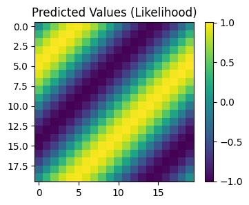
pred_labels = observed_pred.mean.view(n, n)

# Calc abosolute error
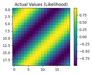
test_y_actual = torch.sin(((test_x[:, 0] + test_x[:, 1]) * (2 * math.pi))).view(n, n)
delta_y = torch.abs(pred_labels - test_y_actual).detach().numpy()

# Define a plotting function
def ax_plot(f, ax, y_labels, title):
    if smoke_test: return  # this is for running the notebook in our testing framework
    im = ax.imshow(y_labels)
    ax.set_title(title)
    f.colorbar(im)

# Plot our predictive means
f, observed_ax = plt.subplots(1, 1, figsize=(4, 3))
ax_plot(f, observed_ax, pred_labels, 'Predicted Values (Likelihood)')

# Plot the true values
f, observed_ax2 = plt.subplots(1, 1, figsize=(4, 3))
ax_plot(f, observed_ax2, test_y_actual, 'Actual Values (Likelihood)')

# Plot the absolute errors
f, observed_ax3 = plt.subplots(1, 1, figsize=(4, 3))
ax_plot(f, observed_ax3, delta_y, 'Absolute Error Surface')