Solving Partial Differential Equation with Q-Exponential Process

Introduction

In this example, we introduce a Bayesian solver to PDE by modeling its solution as a QEP \(u\sim \textrm{q-EP}(0, \mathcal C)\). When choosing a differentiable kernel \(\mathcal C\), the derivatives of the PDE solution, \(\frac{\partial^{\boldsymbol \alpha}}{\partial {\bf x}^{\boldsymbol \alpha}}\), are also QEPs based on the preservation property of linear combination. Assuming a QEP prior, \(\textrm{q-EP}(0, \tilde{\mathcal C})\), for the extended function \(\tilde u = (u, \frac{\partial}{\partial {\bf x}}, \cdots, \frac{\partial^k}{\partial {\bf x}^k})\), we define the likelihood by penalizing the discrepancy between the left-hand side \(P(\tilde u)\) and the right-hand size \(h({\bf x})\) of PDE and approximate the posterior using sparse variational Bayes. See more details in our NIPS2025 paper.

import torch
import qpytorch
import random
import numpy as np
import tqdm
from matplotlib import pyplot as plt

%matplotlib inline

# Setting manual seed for reproducibility
seed=2025
random.seed(seed)
np.random.seed(seed)
torch.manual_seed(seed)
torch.cuda.manual_seed(seed)
torch.cuda.manual_seed_all(seed)
# set device
device = 'cuda' if torch.cuda.is_available() else 'cpu'
print('Using the '+device+' device...')

Using the cpu device...

Burgers’ Equation

We consider the following Burgers’ equation with \(\nu=0.1\):

\begin{align} \frac{\partial}{\partial t} u + u \frac{\partial}{\partial x} u - \nu \frac{\partial^2}{\partial x^2}u &=0, \quad (x, t)\in (-1, 1)\times (0,1], \\ u(x, 0) &= -\sin(\pi x), \quad x \in (-1, 1), \\ u(-1, t) &= u(1,t) = 0, \quad t \in (0,1] . \end{align}

We first create \(25\times 25\) mesh using the following code.

# generate mesh points
def sampled_pts_grid(N_domain, N_boundary, domain, time_dependent = False):
    x1l, x1r = domain[0]
    x2l, x2r = domain[1]

    N_pts = int(torch.sqrt(torch.tensor(N_domain + N_boundary)).item()) - 2
    xx = torch.linspace(x1l, x1r, N_pts + 2)
    yy = torch.linspace(x2l, x2r, N_pts + 2)
    XX, YY = torch.meshgrid(xx, yy, indexing='ij')

    if not time_dependent:

        XX_int = XX[1:-1, 1:-1]
        YY_int = YY[1:-1, 1:-1]

        XXv_bd = torch.cat((XX[:-1, 0], XX[0, :-1], XX[:-1, -1], XX[-1, :-1]))
        YYv_bd = torch.cat((YY[:-1, 0], YY[0, :-1], YY[:-1, -1], YY[-1, :-1]))

    else:

        XX_int = XX[1:-1, 1:]
        YY_int = YY[1:-1, 1:]

        XXv_bd = torch.cat((XX[-1,1:], XX[:, 0], XX[0, 1:]))
        YYv_bd = torch.cat((YY[-1,1:], YY[:, 0], YY[0, 1:]))

    # vectorized (x,y) coordinates
    XXv_int = XX_int.flatten().unsqueeze(1)
    YYv_int = YY_int.flatten().unsqueeze(1)

    XXv_bd = XXv_bd.unsqueeze(1)
    YYv_bd = YYv_bd.unsqueeze(1)

    X_domain = torch.cat((XXv_int, YYv_int), dim=1)
    X_boundary = torch.cat((XXv_bd, YYv_bd), dim=1)
    return X_domain, X_boundary

Now on the mesh with \(N=N_d+N_b\) points of which \(N_d\) are in the domain and \(N_b\) are on the boundary, we have the extended function mu as an \(N\times D\) array where \(D=1+kd\) with max \(k=2\) order derivatives and \(d=2\) physical dimensions. Define the PDE class to specify the left-hand function lhs_f, the right-hand function rhs_f, the boundary condition bdy_g, and extract the solution/derivatives in the domain and on the boundary respectively.

# PDE class
class Burgers(object):
    def __init__(self, alpha=1.0, nu=0.02, domain=np.array([[-1, 1], [0, 1]])):
        self.alpha = alpha
        self.nu = nu
        self.rhs_f = lambda x: torch.zeros(x.shape[0])
        self.bdy_g = lambda x: (-torch.sin(torch.pi*x[:,:-1].squeeze()) * (x[:,-1]==0) + 0*((x[:,0]==1)+(x[:,0]==-1)))
        self.domain = domain
        self.dim = self.domain.shape[0]

    def sampled_pts(self, N_domain, N_boundary, sampled_type='random'):
        Xd, Xb = sampled_pts_grid(N_domain, N_boundary, self.domain, time_dependent=True)
        if sampled_type == 'random':
            Xd += torch.randn(*Xd.shape) * 1e-2
        elif sampled_type == 'grid':
            pass
        self.X_domain = Xd
        self.X_boundary = Xb
        self.Nd, self.Nb = self.X_domain.shape[0], self.X_boundary.shape[0]
        self.rhs = self.rhs_f(self.X_domain)
        self.bdy = self.bdy_g(self.X_boundary)

    def lhs_f(self, u_):
        u_d, u_b, du, d2u_x = self.extract_solution(u_)[0]
        lhs = torch.cat([du[:,-1] + self.alpha*u_d*du[:,:-1].squeeze() - self.nu*d2u_x[:,:self.dim-1].squeeze(),u_b],-1)
        return lhs

    def extract_solution(self, mu, var=None):
        u_d, u_b = mu[...,:self.Nd,0], mu[...,self.Nd:,0]
        du = mu[...,:self.Nd,1:1+self.dim]
        d2u_x = mu[...,:self.Nd,1+self.dim:]
        if var is None: var = torch.ones_like(mu)
        v_d, v_b = var[...,:self.Nd,0], var[...,self.Nd:,0]
        dv = var[...,:self.Nd,1:1+self.dim]
        d2v_x = var[...,:self.Nd,1+self.dim:]
        return [u_d, u_b, du, d2u_x], [v_d, v_b, dv, d2v_x]

    def plot_solution(self, u, ax=None, **kwargs):
        import matplotlib.pyplot as plt
        x, t = self.X_domain[:,0], self.X_domain[:,1]
        N_pts = int(np.sqrt(self.Nd+self.Nb))-2
        x = x.reshape((N_pts,N_pts+1))
        t = t.reshape((N_pts,N_pts+1))
        if ax is None:
            ax = plt.gca()
        ctf = ax.contourf(x, t , u, **kwargs)
        clb = plt.colorbar(ctf, ax=ax)
        clb.ax.tick_params(labelsize = ax.yaxis.get_tick_params()['labelsize'])

# generate PDE
alpha = 1.0
nu = 0.1
domain=np.array([[-1, 1], [0, 1]])
N_dom, N_bdy = 625, 100
burgers = Burgers(alpha, nu, domain)
burgers.sampled_pts(N_dom, N_bdy, sampled_type='grid')
burgers_X = torch.cat([burgers.X_domain,burgers.X_boundary]).type(torch.float).to(device)
lims = torch.from_numpy(domain.T)

Reference solution

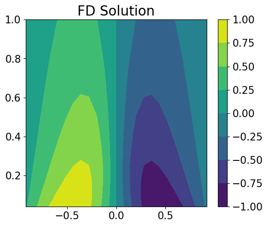
As a reference, we solve the Burgers’ equation using highly-resolved finite difference method with Cole-Hopf transformation.

# Solve Burgers' equation using finite difference method.
def u_truth(t, x, nu=0.02):
    [Gauss_pts, weights] = np.polynomial.hermite.hermgauss(80)
    temp = x - np.sqrt(4 * nu * t) * Gauss_pts
    val1 = weights * np.sin(np.pi * temp) * np.exp(-np.cos(np.pi * temp) / (2 * np.pi * nu))
    val2 = weights * np.exp(-np.cos(np.pi * temp) / (2 * np.pi * nu))
    return - val1.sum(axis=1) / val2.sum(axis=1)

def solve_Burgers(n, nu=0.02):
    t = np.linspace(0, 1, n+2)
    x = np.linspace(-1, 1, n+2)
    tt, xx = np.meshgrid(t, x)
    tx = np.vstack([tt.flatten(), xx.flatten()])
    u = u_truth(tx[0].reshape(-1, 1), tx[1].reshape(-1, 1), nu)
    return np.stack([tt, xx, u.reshape(n+2, n+2)])

N_pts = int(np.sqrt(burgers.Nd+burgers.Nb))-2
txu = solve_Burgers(N_pts, nu)
txu = txu[:, 1:-1, 1:]
u_FD = txu[2]

# plot
plt.figure(figsize=(6,5))
plt.tick_params(axis='both', which='major', labelsize=15)
plt.contourf(txu[1], txu[0], u_FD)#, 50)#, cmap='inferno')
clb = plt.colorbar()
clb.ax.tick_params(labelsize=15)
plt.title("FD Solution", fontsize=20)

None

Setting up the model

We model the extended function \(\tilde u\) using some variational distribution \(\textrm{q-ED}(\mu, \Sigma)\). With nonlinear left-hand side function \(P\), \(P(\tilde u)\) no longer follows q-exponential distribution. QPyTorch has PDESolver model to propagate the variational distribution \(\textrm{q-ED}(\mu, \Sigma)\) through the PDE by linearizing \(P\):

\begin{align} P(\tilde{u}) &\approx P(\tilde{u}_0) + \nabla P(\tilde{u}_0)(\tilde{u}-\tilde{u}_0) \sim \textrm{q-ED}(\mu_*, \Sigma_*), \\ \mu_* &= P(\tilde{u}_0) + \nabla P(\tilde{u}_0)(\mu-\tilde{u}_0), \quad \Sigma_* = P(\tilde{u}_0) \Sigma P(\tilde{u}_0)^{\mathsf T} + \delta I. \end{align} where the reference point can be chosen as \(\tilde{u}_0=\mu\), and \(\delta>0\) is a small nugget added to make the propagated covariance postive definite.

The PDESolver class inherits from ApproximateQEP to approximate the posterior with sparse variatinoal Bayes. To faciliate modeling derivatives and differential equations, QPyTorch defines new methods including Matern32KernelGrad, Matern52KernelGradGrad, RQKernelGrad, and RQKernelGradGrad which are not available in GPyTorch.

# QEP solver
POWER = 1.0
class QEPsolver(qpytorch.models.PDESolver):
        def __init__(self, pde_lhs, power=torch.tensor(1.0), num_inducing=256):
            self.power = power
            input_dims = burgers.dim
            output_dims = input_dims*2

            # inducing_points = lims[0] + torch.rand(num_inducing, input_dims) * lims.diff(dim=0)
            inducing_points = burgers_X[torch.randperm(burgers_X.size(0))[:num_inducing]]
            batch_shape = torch.Size([output_dims])
            variational_distribution = qpytorch.variational.NaturalVariationalDistribution(
                num_inducing_points=num_inducing,
                batch_shape=batch_shape,
                power=self.power
            )
            variational_strategy = qpytorch.variational.MultitaskVariationalStrategy(
                self,
                inducing_points,
                variational_distribution,
                learn_inducing_locations=True,
                # jitter_val = 1.0e-4
            )

            super().__init__(pde_lhs, variational_strategy)
            # self.mean_module = qpytorch.means.ConstantMeanGradGrad()
            self.mean_module = qpytorch.means.LinearMeanGradGrad(input_dims)
            # self.base_kernel = qpytorch.kernels.RBFKernelGradGrad(ard_num_dims=input_dims, interleaved=False)
            # self.base_kernel = qpytorch.kernels.RQKernelGradGrad(ard_num_dims=input_dims, interleaved=False)
            self.base_kernel = qpytorch.kernels.Matern52KernelGradGrad(ard_num_dims=input_dims, eps=1e-4, interleaved=False)
            self.covar_module = qpytorch.kernels.ScaleKernel(self.base_kernel)
            self.covar_module.base_kernel.register_constraint("raw_lengthscale", qpytorch.constraints.Interval(1e-2, 1))

        def forward(self, x):
            N = x.shape[-2]
            mean_x = self.mean_module(x) # ... x N x (2D+1)
            covar_x = self.covar_module(x)# ... x N(2D+1) x N(2D+1)
            mean_x = mean_x[...,:-1]
            covar_x = covar_x[...,:-N,:-N]
            return qpytorch.distributions.MultitaskMultivariateQExponential(mean_x, covar_x, power=self.power, interleaved=False)

        def predict(self, testX):
            with torch.no_grad():
                output = self(testX)
                if type(likelihood) is qpytorch.likelihoods.QExponentialLikelihood:
                    output = output.to_data_uncorrelated_dist()
                predictions = likelihood(output)
                pred_m = predictions.mean
                pred_v = predictions.variance
                if pred_m.ndim == 3: pred_m = pred_m.mean(0)
                if pred_v.ndim == 3: pred_v = pred_v.mean(0)
            return pred_m, pred_v

# likelihood
likelihood = qpytorch.likelihoods.QExponentialLikelihood(power=torch.tensor(POWER), noise_constraint=qpytorch.constraints.Interval(1e-2,1.0))
likelihood.noise = torch.tensor(0.02)
# define the model
model = QEPsolver(pde_lhs=burgers.lhs_f, power=torch.tensor(POWER))
model.covar_module.base_kernel.lengthscale = torch.tensor([.25,.5] if POWER>1.0 else [0.15, 0.2])
# set device
model = model.to(device)
likelihood = likelihood.to(device)

Training

We use the variational inference with natural gradient descent as in this NGD example.

# this is for running the notebook in our testing framework
import os
smoke_test = ('CI' in os.environ)
num_iter = 2 if smoke_test else 200

# "Loss" for QEPs - the marginal log likelihood
mll = qpytorch.mlls.VariationalELBO(likelihood, model, num_data=burgers.Nd+burgers.Nb)

# Use the adam optimizer
variational_ngd_optimizer = qpytorch.optim.NGD(model.variational_parameters(), num_data=burgers.Nd+burgers.Nb, lr=0.01)
hyperparameter_optimizer = torch.optim.Adam([
    {'params': model.hyperparameters()},
    {'params': likelihood.parameters()},
], lr=0.001)

# Find optimal model hyperparameters
model.train()
likelihood.train()

iterator = tqdm.notebook.tqdm(range(num_iter))
for i in iterator:
    variational_ngd_optimizer.zero_grad()
    hyperparameter_optimizer.zero_grad()
    with qpytorch.settings.cholesky_jitter(double_value=1e-3):
        output = model(burgers_X)
        u0 = output.mean.detach().clone()
        ppgt_dist = model.propagate(output, u0, interleaved=model.base_kernel._interleaved)
        loss = -mll(ppgt_dist, torch.cat([burgers.rhs, burgers.bdy],-1).to(device)).sum()
    loss.backward()
    iterator.set_postfix(loss=loss.item(), lengthscales=model.covar_module.base_kernel.lengthscale.detach().numpy(), noise=likelihood.noise.item())
    # print("Iter %d/%d - Loss: %.3f   lengthscales: %.3f, %.3f   noise: %.3f" % (
    #     i + 1, training_iter, loss.item(),
    #     model.covar_module.base_kernel.lengthscale.squeeze()[0].mean(),
    #     model.covar_module.base_kernel.lengthscale.squeeze()[1].mean(),
    #     likelihood.noise.item()
    # ))
    variational_ngd_optimizer.step()
    hyperparameter_optimizer.step()

/Users/shiweilan/Projects/QPyTorch/qpytorch/distributions/multivariate_qexponential.py:475: NumericalWarning: Negative variance values detected. This is likely due to numerical instabilities. Rounding negative variances up to 1e-06.
  warnings.warn(

Prediction

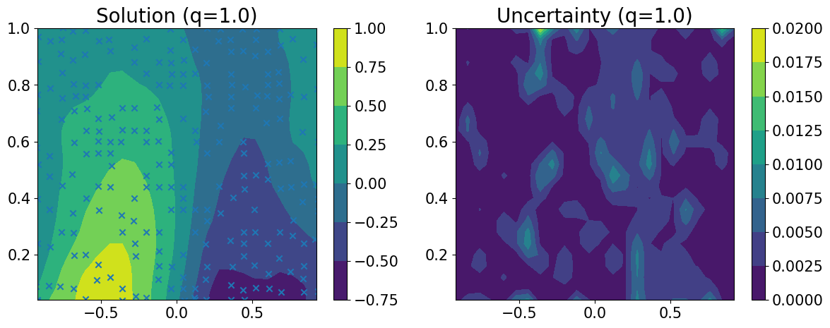
Model predictions are also similar to QEP regression, but we have the uncertainty of the solution at the same time.

# Set into eval mode
model.eval()
likelihood.eval()

# prepare quantites to plot
pred1_m, pred1_v = output.mean, output.variance
N_pts = int(np.sqrt(burgers.Nd+burgers.Nb))-2

# Initialize plots
fig, axes = plt.subplots(1,2, figsize=(14,5))

# solution
u = burgers.extract_solution(pred1_m)[0][0].detach().cpu()
axes.flat[0].tick_params(axis='both', which='major', labelsize=15)
burgers.plot_solution(u.reshape((N_pts,N_pts+1)), ax=axes.flat[0])#, levels=50)
induc_pts = model.variational_strategy.inducing_points.detach().cpu()
axes.flat[0].autoscale(False)
axes.flat[0].scatter(induc_pts[:,0],induc_pts[:,1], marker='x')
axes.flat[0].set_title('Solution (q='+str(round(POWER,1))+')', fontsize=20)
# uncertainty
v = burgers.extract_solution(pred1_v)[0][0].detach().cpu()
axes.flat[1].tick_params(axis='both', which='major', labelsize=15)
burgers.plot_solution(v.reshape((N_pts,N_pts+1)), ax=axes.flat[1])#, levels=50)
axes.flat[1].set_title('Uncertainty (q='+str(round(POWER,1))+')', fontsize=20)

None

One can try for longer time to obtain solution with improved precision. Refer to the NIPS2025 paper.