Batch Uncorrelated Multioutput QEP

Introduction

This notebook demonstrates how to wrap uncorrelated QEP models into a convenient Multi-Output QEP model. It uses batch dimensions for efficient computation. Unlike in the Multitask QEP Example, this do not model correlations between outcomes, but treats outcomes independently.

This type of model is useful if - when the number of training / test points is equal for the different outcomes - using the same covariance modules and / or likelihoods for each outcome

For non-block designs (i.e. when the above points do not apply), you should instead use a ModelList QEP as described in the ModelList multioutput example.

import math
import torch
import qpytorch
from matplotlib import pyplot as plt

%matplotlib inline

Set up training data

In the next cell, we set up the training data for this example. We’ll be using 100 regularly spaced points on [0,1] which we evaluate the function on and add Gaussian noise to get the training labels.

We’ll have two functions - a sine function (y1) and a cosine function (y2).

For MTGPs, our train_targets will actually have two dimensions: with the second dimension corresponding to the different tasks.

train_x = torch.linspace(0, 1, 100)

train_y = torch.stack([
    torch.sin(train_x * (2 * math.pi)) + torch.randn(train_x.size()) * 0.2,
    torch.cos(train_x * (2 * math.pi)) + torch.randn(train_x.size()) * 0.2,
], -1)

Define a batch QEP model

The model should be somewhat similar to the ExactQEP model in the simple regression example. The differences:

1. The model will use the batch dimension to learn multiple uncorrelated QEPs simultaneously.

2. We’re going to give the mean and covariance modules a batch_shape argument. This allows us to learn different hyperparameters for each model.

3. The model will return a MultitaskMultivariateQExponential distribution rather than a MultivariateQExponential. We will construct this distribution to convert the batch dimensions into distinct outputs.

POWER = 1.0
class BatchUncorrelatedMultitaskQEPModel(qpytorch.models.ExactQEP):
    def __init__(self, train_x, train_y, likelihood):
        super().__init__(train_x, train_y, likelihood)
        self.power = torch.tensor(POWER)
        self.mean_module = qpytorch.means.ConstantMean(batch_shape=torch.Size([2]))
        self.covar_module = qpytorch.kernels.ScaleKernel(
            qpytorch.kernels.RBFKernel(batch_shape=torch.Size([2])),
            batch_shape=torch.Size([2])
        )

    def forward(self, x):
        mean_x = self.mean_module(x)
        covar_x = self.covar_module(x)
        return qpytorch.distributions.MultitaskMultivariateQExponential.from_batch_qep(
            qpytorch.distributions.MultivariateQExponential(mean_x, covar_x, power=self.power)
        )


likelihood = qpytorch.likelihoods.MultitaskQExponentialLikelihood(num_tasks=2, power=torch.tensor(POWER))
model = BatchUncorrelatedMultitaskQEPModel(train_x, train_y, likelihood)

Train the model hyperparameters

# this is for running the notebook in our testing framework
import os
smoke_test = ('CI' in os.environ)
training_iterations = 2 if smoke_test else 80


# Find optimal model hyperparameters
model.train()
likelihood.train()

# Use the adam optimizer
optimizer = torch.optim.Adam(model.parameters(), lr=0.1)  # Includes QExponentialLikelihood parameters

# "Loss" for QEPs - the marginal log likelihood
mll = qpytorch.mlls.ExactMarginalLogLikelihood(likelihood, model)

for i in range(training_iterations):
    optimizer.zero_grad()
    output = model(train_x)
    loss = -mll(output, train_y)
    loss.backward()
    print('Iter %d/%d - Loss: %.3f' % (i + 1, training_iterations, loss.item()))
    optimizer.step()

Iter 1/80 - Loss: 2.100
Iter 2/80 - Loss: 2.058
Iter 3/80 - Loss: 2.012
Iter 4/80 - Loss: 1.961
Iter 5/80 - Loss: 1.906
Iter 6/80 - Loss: 1.847
Iter 7/80 - Loss: 1.785
Iter 8/80 - Loss: 1.721
Iter 9/80 - Loss: 1.656
Iter 10/80 - Loss: 1.595
Iter 11/80 - Loss: 1.540
Iter 12/80 - Loss: 1.493
Iter 13/80 - Loss: 1.455
Iter 14/80 - Loss: 1.423
Iter 15/80 - Loss: 1.394
Iter 16/80 - Loss: 1.369
Iter 17/80 - Loss: 1.345
Iter 18/80 - Loss: 1.324
Iter 19/80 - Loss: 1.303
Iter 20/80 - Loss: 1.284
Iter 21/80 - Loss: 1.265
Iter 22/80 - Loss: 1.246
Iter 23/80 - Loss: 1.228
Iter 24/80 - Loss: 1.209
Iter 25/80 - Loss: 1.190
Iter 26/80 - Loss: 1.170
Iter 27/80 - Loss: 1.151
Iter 28/80 - Loss: 1.131
Iter 29/80 - Loss: 1.110
Iter 30/80 - Loss: 1.089
Iter 31/80 - Loss: 1.068
Iter 32/80 - Loss: 1.046
Iter 33/80 - Loss: 1.024
Iter 34/80 - Loss: 1.002
Iter 35/80 - Loss: 0.979
Iter 36/80 - Loss: 0.956
Iter 37/80 - Loss: 0.934
Iter 38/80 - Loss: 0.911
Iter 39/80 - Loss: 0.888
Iter 40/80 - Loss: 0.865
Iter 41/80 - Loss: 0.842
Iter 42/80 - Loss: 0.820
Iter 43/80 - Loss: 0.798
Iter 44/80 - Loss: 0.776
Iter 45/80 - Loss: 0.754
Iter 46/80 - Loss: 0.732
Iter 47/80 - Loss: 0.710
Iter 48/80 - Loss: 0.689
Iter 49/80 - Loss: 0.669
Iter 50/80 - Loss: 0.648
Iter 51/80 - Loss: 0.628
Iter 52/80 - Loss: 0.608
Iter 53/80 - Loss: 0.589
Iter 54/80 - Loss: 0.569
Iter 55/80 - Loss: 0.550
Iter 56/80 - Loss: 0.531
Iter 57/80 - Loss: 0.513
Iter 58/80 - Loss: 0.494
Iter 59/80 - Loss: 0.476
Iter 60/80 - Loss: 0.458
Iter 61/80 - Loss: 0.440
Iter 62/80 - Loss: 0.423
Iter 63/80 - Loss: 0.406
Iter 64/80 - Loss: 0.389
Iter 65/80 - Loss: 0.372
Iter 66/80 - Loss: 0.356
Iter 67/80 - Loss: 0.341
Iter 68/80 - Loss: 0.325
Iter 69/80 - Loss: 0.311
Iter 70/80 - Loss: 0.296
Iter 71/80 - Loss: 0.282
Iter 72/80 - Loss: 0.268
Iter 73/80 - Loss: 0.255
Iter 74/80 - Loss: 0.243
Iter 75/80 - Loss: 0.230
Iter 76/80 - Loss: 0.218
Iter 77/80 - Loss: 0.207
Iter 78/80 - Loss: 0.196
Iter 79/80 - Loss: 0.186
Iter 80/80 - Loss: 0.175

Make predictions with the model

# Set into eval mode
model.eval()
likelihood.eval()

# Initialize plots
f, (y1_ax, y2_ax) = plt.subplots(1, 2, figsize=(8, 3))

# Make predictions
with torch.no_grad(), qpytorch.settings.fast_pred_var():
    test_x = torch.linspace(0, 1, 51)
    predictions = likelihood(model(test_x))
    mean = predictions.mean
    lower, upper = predictions.confidence_region(rescale=True)

# This contains predictions for both tasks, flattened out
# The first half of the predictions is for the first task
# The second half is for the second task

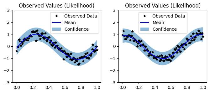
# Plot training data as black stars
y1_ax.plot(train_x.detach().numpy(), train_y[:, 0].detach().numpy(), 'k*')
# Predictive mean as blue line
y1_ax.plot(test_x.numpy(), mean[:, 0].numpy(), 'b')
# Shade in confidence
y1_ax.fill_between(test_x.numpy(), lower[:, 0].numpy(), upper[:, 0].numpy(), alpha=0.5)
y1_ax.set_ylim([-3, 3])
y1_ax.legend(['Observed Data', 'Mean', 'Confidence'])
y1_ax.set_title('Observed Values (Likelihood)')

# Plot training data as black stars
y2_ax.plot(train_x.detach().numpy(), train_y[:, 1].detach().numpy(), 'k*')
# Predictive mean as blue line
y2_ax.plot(test_x.numpy(), mean[:, 1].numpy(), 'b')
# Shade in confidence
y2_ax.fill_between(test_x.numpy(), lower[:, 1].numpy(), upper[:, 1].numpy(), alpha=0.5)
y2_ax.set_ylim([-3, 3])
y2_ax.legend(['Observed Data', 'Mean', 'Confidence'])
y2_ax.set_title('Observed Values (Likelihood)')

None