Q-Exponential Process Latent Variable Models (QEPLVM) with SVI
Vidhi Lalchand, 2021
Introduction
In this notebook we demonstrate the QEPLVM model class introduced in Lawrence, 2005 and its Bayesian incarnation introduced in Titsias & Lawrence, 2010.
QEPLVMs use q-exponential processes in an unsupervised context, where a low dimensional representation of the data (\(X \equiv \{\mathbf{x}_{n}\}_{n=1}^{N}\in \mathbb{R}^{N \times Q}\)) is learnt given some high dimensional real valued observations \(Y \equiv \{\mathbf{y}_{n}\}_{n=1}^{N} \in \mathbb{R}^{N \times D}\). \(Q < D\) provides dimensionality reduction. The forward mapping (\(X \longrightarrow Y\)) is governed by QEPs independently defined across dimensions \(D\). Q (the dimensionality of the latent space is usually fixed before hand).
One can either learn point estimates for each \(\mathbf{x}_{n}\) by maximizing the QEP marginal likelihood jointly wrt. the kernel hyperparameters \(\theta\) and the latent inputs \(\mathbf{x}_{n}\). Alternatively, one can variationally integrate out \(X\) by using the sparse variational formulation where a variational distribution \(q(X) = \prod_{n=1}^{N}\mathcal{Q}(\mathbf{x}_{n}; \mu_{n}, s_{n}\mathbb{I}_{Q})\). This tutorial focuses on the latter.
The probabilistic model is:
\begin{align*} \textrm{ Prior on latents: } p(X) &= \displaystyle \prod _{n=1}^N \mathcal{Q} (\mathbf{x}_{n};\mathbf{0}, \mathbb{I}_{Q}),\\ \textrm{Prior on mapping: } p(\mathbf{f}|X, \mathbf{\theta}) &= \displaystyle \prod_{d=1}^{D}\mathcal{Q}(\mathbf{f}_{d}; \mathbf{0}, K_{ff}^{(d)}),\\ \textrm{Data likelihood: } p(Y| \mathbf{f}, X) &= \prod_{n=1}^N \prod_{d=1}^D \mathcal{Q}(y_{n,d}; \mathbf{f}_{d}(\mathbf{x}_{n}), \sigma^{2}_{y}), \end{align*}
[1]:
# Standard imports
import matplotlib.pylab as plt
import torch
import os
import numpy as np
from pathlib import Path

# If you are running this notebook interactively
wdir = Path(os.path.abspath('')).parent.parent
os.chdir(wdir)

# qpytorch imports
from qpytorch.mlls import VariationalELBO
from qpytorch.priors import QExponentialPrior

%matplotlib inline

# Setting manual seed for reproducibility
torch.manual_seed(73)
np.random.seed(73)

# this is for running the notebook in our testing framework
smoke_test = ('CI' in os.environ)
Set up training data
We use the canonical multi-phase oilflow dataset used in Titsias & Lawrence, 2010 that consists of 1000, 12 dimensional observations belonging to three known classes corresponding to different phases of oilflow.
[2]:
# import urllib.request
import tarfile

# url = "http://staffwww.dcs.shef.ac.uk/people/N.Lawrence/resources/3PhData.tar.gz"
# urllib.request.urlretrieve(url, '3PhData.tar.gz')
with tarfile.open('./examples/045_QEPLVM/3PhData.tar.gz', 'r') as f:
    f.extract('DataTrn.txt')
    f.extract('DataTrnLbls.txt')

Y = torch.Tensor(np.loadtxt(fname='DataTrn.txt'))
labels = torch.Tensor(np.loadtxt(fname='DataTrnLbls.txt'))
labels = (labels @ np.diag([1, 2, 3])).sum(axis=1)
Defining the QEPLVM model
We will be using the BayesianQEPLVM model class which is compatible with three different modes of inference.
Point estimate for the latent variables \(X \equiv \{x_{n}\}_{n=1}^{N}\).
MAP estimate for the latent variables where we have an additional log prior term in the ELBO.
Variational distribution \(q(x_{n})\) corresponding to latent variables.
The latent variable ELBO for (c) is given by:
The latent variable ELBO corresponding to (a) just has the first two terms and corresponding to (b) includes the log prior for latent variables \(p(\mathbf{x}_{n})\) in the ELBO.
This ELBO is optimised w.r.t local variational parameters \(\phi\), global variational parameters \(\lambda\), kernel hyperparameters \(\theta\) and likelihood noise \(\sigma^{y}\).
The BayesianQEPLVM is built on top of the Sparse QEP formulation. Similar to the SVQEP example, we’ll use a CholeskyVariationalDistribution to model \(q(\mathbf{u})\) and the standard VariationalStrategy as defined by Hensman et al. (2015).
[3]:
from qpytorch.models.qeplvm.latent_variable import *
from qpytorch.models.qeplvm.bayesian_qeplvm import BayesianQEPLVM
from matplotlib import pyplot as plt
from tqdm.notebook import trange
from qpytorch.means import ZeroMean
from qpytorch.mlls import VariationalELBO
from qpytorch.priors import QExponentialPrior
from qpytorch.likelihoods import QExponentialLikelihood
from qpytorch.variational import VariationalStrategy
from qpytorch.variational import CholeskyVariationalDistribution
from qpytorch.kernels import ScaleKernel, RBFKernel
from qpytorch.distributions import MultivariateQExponential
POWER = 1.0

def _init_pca(Y, latent_dim):
    U, S, V = torch.pca_lowrank(Y, q = latent_dim)
    return torch.nn.Parameter(torch.matmul(Y, V[:,:latent_dim]))


class bQEPLVM(BayesianQEPLVM):
    def __init__(self, n, data_dim, latent_dim, n_inducing, pca=False):
        self.power = torch.tensor(POWER)
        self.n = n
        self.batch_shape = torch.Size([data_dim])

        # Locations Z_{d} corresponding to u_{d}, they can be randomly initialized or
        # regularly placed with shape (D x n_inducing x latent_dim).
        self.inducing_inputs = torch.randn(data_dim, n_inducing, latent_dim)

        # Sparse Variational Formulation (inducing variables initialised as randn)
        q_u = CholeskyVariationalDistribution(n_inducing, batch_shape=self.batch_shape, power=self.power)
        q_f = VariationalStrategy(self, self.inducing_inputs, q_u, learn_inducing_locations=True)

        # Define prior for X
        X_prior_mean = torch.zeros(n, latent_dim)  # shape: N x Q
        prior_x = QExponentialPrior(X_prior_mean, torch.ones_like(X_prior_mean), power=self.power)

        # Initialise X with PCA or randn
        if pca == True:
             X_init = _init_pca(Y, latent_dim) # Initialise X to PCA
        else:
             X_init = torch.nn.Parameter(torch.randn(n, latent_dim))

        # LatentVariable (c)
        X = VariationalLatentVariable(n, data_dim, latent_dim, X_init, prior_x)

        # For (a) or (b) change to below:
        # X = PointLatentVariable(n, latent_dim, X_init)
        # X = MAPLatentVariable(n, latent_dim, X_init, prior_x)

        super().__init__(X, q_f)

        # Kernel (acting on latent dimensions)
        self.mean_module = ZeroMean(ard_num_dims=latent_dim)
        self.covar_module = ScaleKernel(RBFKernel(ard_num_dims=latent_dim))

    def forward(self, X):
        mean_x = self.mean_module(X)
        covar_x = self.covar_module(X)
        dist = MultivariateQExponential(mean_x, covar_x, power=self.power)
        return dist

    def _get_batch_idx(self, batch_size):
        valid_indices = np.arange(self.n)
        batch_indices = np.random.choice(valid_indices, size=batch_size, replace=False)
        return np.sort(batch_indices)
Training the model
While we need to specify the dimensionality of the latent variables at the outset, one of the advantages of the Bayesian framework is that by using a ARD kernel we can prune dimensions corresponding to small inverse lengthscales.
[4]:
N = len(Y)
data_dim = Y.shape[1]
latent_dim = data_dim
n_inducing = 25
pca = False

# Model
model = bQEPLVM(N, data_dim, latent_dim, n_inducing, pca=pca)

# Likelihood
likelihood = QExponentialLikelihood(batch_shape=model.batch_shape, power=model.power)

# Declaring the objective to be optimised along with optimiser
# (see models/latent_variable.py for how the additional loss terms are accounted for)
mll = VariationalELBO(likelihood, model, num_data=len(Y))

optimizer = torch.optim.Adam([
    {'params': model.parameters()},
    {'params': likelihood.parameters()}
], lr=0.01)
We use mini-batch training for scalability where only a subset of the local variaitonal params are optimised in each iteration.
[5]:
# Training loop - optimises the objective wrt kernel hypers, variational params and inducing inputs
# using the optimizer provided.

loss_list = []
iterator = trange(10000 if not smoke_test else 4, leave=True)
batch_size = 100
for i in iterator:
    batch_index = model._get_batch_idx(batch_size)
    optimizer.zero_grad()
    sample = model.sample_latent_variable()  # a full sample returns latent x across all N
    sample_batch = sample[batch_index]
    output_batch = model(sample_batch)
    loss = -mll(output_batch, Y[batch_index].T).sum()
    loss_list.append(loss.item())
    iterator.set_description('Loss: ' + str(float(np.round(loss.item(),2))) + ", iter no: " + str(i))
    loss.backward()
    optimizer.step()
Visualising the 2d latent subspace
Visualising a two dimensional slice of the latent space corresponding to the most dominant latent dimensions.
[6]:
inv_lengthscale = 1 / model.covar_module.base_kernel.lengthscale
values, indices = torch.topk(model.covar_module.base_kernel.lengthscale, k=2,largest=False)

l1 = indices.numpy().flatten()[0]
l2 = indices.numpy().flatten()[1]

plt.figure(figsize=(20, 8))
colors = ['r', 'b', 'g']

plt.subplot(131)
X = model.X.q_mu.detach().numpy()
std = torch.nn.functional.softplus(model.X.q_log_sigma).detach().numpy()
plt.title('2d latent subspace corresponding to 3 phase oilflow', fontsize='small')
plt.xlabel('Latent dim 1')
plt.ylabel('Latent dim 2')

# Select index of the smallest lengthscales by examining model.covar_module.base_kernel.lengthscales
for i, label in enumerate(np.unique(labels)):
    X_i = X[labels == label]
    scale_i = std[labels == label]
    plt.scatter(X_i[:, l1], X_i[:, l2], c=[colors[i]], label=label)
    plt.errorbar(X_i[:, l1], X_i[:, l2], xerr=scale_i[:,l1], yerr=scale_i[:,l2], label=label,c=colors[i], fmt='none')

plt.subplot(132)
plt.bar(np.arange(latent_dim), height=inv_lengthscale.detach().numpy().flatten())
plt.title('Inverse Lengthscale with SE-ARD kernel', fontsize='small')

plt.subplot(133)
plt.plot(loss_list, label='batch_size=100')
plt.title('Neg. ELBO Loss', fontsize='small')
None
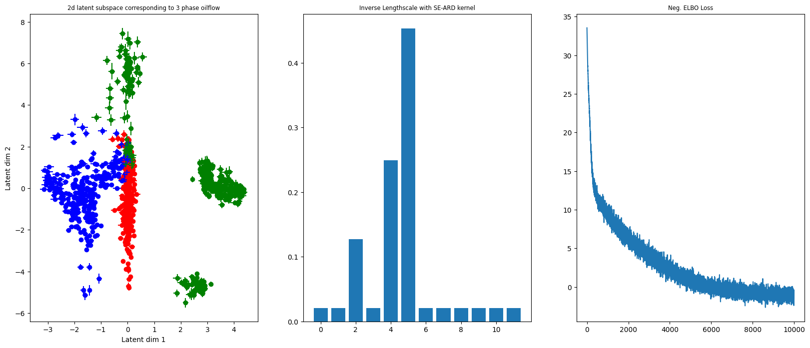
The vertical and horizontal bars indicate axis aligned q-exponential uncertainty around each latent point.