Spectral QEP Learning with Deltas
In this paper, we demonstrate another approach to spectral learning with QEPs, learning a spectral density as a simple mixture of deltas. This has been explored, for example, as early as Lázaro-Gredilla et al., 2010.
[1]:
import qpytorch
import torch
Load Data
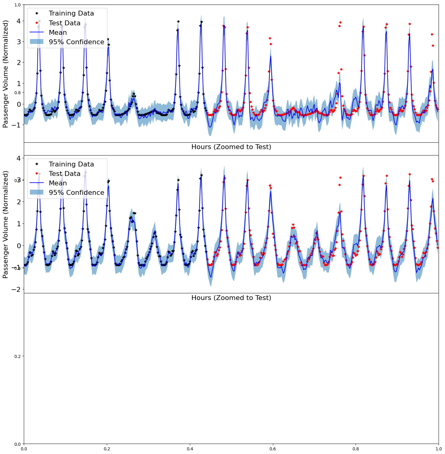
For this notebook, we’ll be using a sample set of timeseries data of BART ridership on the 5 most commonly traveled stations in San Francisco. This subsample of data was selected and processed from Pyro’s examples http://docs.pyro.ai/en/stable/_modules/pyro/contrib/examples/bart.html
[2]:
import os
import urllib.request

smoke_test = ('CI' in os.environ)

if not smoke_test and not os.path.isfile('../BART_sample.pt'):
    print('Downloading \'BART\' sample dataset...')
    urllib.request.urlretrieve('https://drive.google.com/uc?export=download&id=1A6LqCHPA5lHa5S3lMH8mLMNEgeku8lRG', '../BART_sample.pt')
    torch.manual_seed(1)

if smoke_test:
    train_x, train_y, test_x, test_y = torch.randn(2, 100, 1), torch.randn(2, 100), torch.randn(2, 100, 1), torch.randn(2, 100)
else:
    train_x, train_y, test_x, test_y = torch.load('../BART_sample.pt', map_location='cpu')

if torch.cuda.is_available():
    train_x, train_y, test_x, test_y = train_x.cuda(), train_y.cuda(), test_x.cuda(), test_y.cuda()

print(train_x.shape, train_y.shape, test_x.shape, test_y.shape)
torch.Size([5, 1440, 1]) torch.Size([5, 1440]) torch.Size([5, 240, 1]) torch.Size([5, 240])
[3]:
train_x_min = train_x.min()
train_x_max = train_x.max()

train_x = train_x - train_x_min
test_x = test_x - train_x_min

train_y_mean = train_y.mean(dim=-1, keepdim=True)
train_y_std = train_y.std(dim=-1, keepdim=True)

train_y = (train_y - train_y_mean) / train_y_std

test_y = (test_y - train_y_mean) / train_y_std
Define a Model
The only thing of note here is the use of the kernel. For this example, we’ll learn a kernel with 2048 deltas in the mixture, and initialize by sampling directly from the empirical spectrum of the data.
[4]:
POWER = 1.0
class SpectralDeltaQEP(qpytorch.models.ExactQEP):
    def __init__(self, train_x, train_y, num_deltas, noise_init=None):
        self.power = torch.tensor(POWER)
        likelihood = qpytorch.likelihoods.QExponentialLikelihood(noise_constraint=qpytorch.constraints.GreaterThan(1e-11), power=self.power)
        likelihood.register_prior("noise_prior", qpytorch.priors.HorseshoePrior(0.1), "noise")
        likelihood.noise = 1e-2

        super(SpectralDeltaQEP, self).__init__(train_x, train_y, likelihood)
        self.mean_module = qpytorch.means.ConstantMean()
        base_covar_module = qpytorch.kernels.SpectralDeltaKernel(
            num_dims=train_x.size(-1),
            num_deltas=num_deltas,
        )
        base_covar_module.initialize_from_data(train_x[0], train_y[0])
        self.covar_module = qpytorch.kernels.ScaleKernel(base_covar_module)

    def forward(self, x):
        mean_x = self.mean_module(x)
        covar_x = self.covar_module(x)
        return qpytorch.distributions.MultivariateQExponential(mean_x, covar_x, power=self.power)
[5]:
model = SpectralDeltaQEP(train_x, train_y, num_deltas=1500)

if torch.cuda.is_available():
    model = model.cuda()
Train
[6]:
model.train()
mll = qpytorch.mlls.ExactMarginalLogLikelihood(model.likelihood, model)
optimizer = torch.optim.Adam(model.parameters(), lr=0.01)
scheduler = torch.optim.lr_scheduler.MultiStepLR(optimizer=optimizer, milestones=[40])

num_iters = 1000 if not smoke_test else 4

with qpytorch.settings.max_cholesky_size(0):  # Ensure we dont try to use Cholesky
    for i in range(num_iters):
        optimizer.zero_grad()
        output = model(train_x)
        loss = -mll(output, train_y)
        if train_x.dim() == 3:
            loss = loss.mean()
        loss.backward()
        optimizer.step()

        if i % 10 == 0:
            print(f'Iteration {i} - loss = {loss:.2f} - noise = {model.likelihood.noise.item():e}')

        scheduler.step()
Iteration 0 - loss = 2.13 - noise = 9.900989e-03
Iteration 10 - loss = 2.17 - noise = 9.134914e-03
Iteration 20 - loss = 1.94 - noise = 8.356065e-03
Iteration 30 - loss = 1.90 - noise = 7.500547e-03
Iteration 40 - loss = 1.81 - noise = 6.778868e-03
Iteration 50 - loss = 1.71 - noise = 6.703777e-03
Iteration 60 - loss = 1.64 - noise = 6.623809e-03
Iteration 70 - loss = 1.57 - noise = 6.541504e-03
Iteration 80 - loss = 1.54 - noise = 6.456869e-03
Iteration 90 - loss = 1.52 - noise = 6.373539e-03
Iteration 100 - loss = 1.51 - noise = 6.291725e-03
Iteration 110 - loss = 1.48 - noise = 6.212601e-03
Iteration 120 - loss = 1.48 - noise = 6.135635e-03
Iteration 130 - loss = 1.44 - noise = 6.060692e-03
Iteration 140 - loss = 1.45 - noise = 5.986421e-03
Iteration 150 - loss = 1.43 - noise = 5.913956e-03
Iteration 160 - loss = 1.42 - noise = 5.843284e-03
Iteration 170 - loss = 1.40 - noise = 5.773738e-03
Iteration 180 - loss = 1.35 - noise = 5.704680e-03
Iteration 190 - loss = 1.37 - noise = 5.633501e-03
Iteration 200 - loss = 1.34 - noise = 5.562404e-03
Iteration 210 - loss = 1.35 - noise = 5.493562e-03
Iteration 220 - loss = 1.34 - noise = 5.426683e-03
Iteration 230 - loss = 1.34 - noise = 5.360365e-03
Iteration 240 - loss = 1.32 - noise = 5.295387e-03
Iteration 250 - loss = 1.30 - noise = 5.232106e-03
Iteration 260 - loss = 1.34 - noise = 5.170099e-03
Iteration 270 - loss = 1.31 - noise = 5.109232e-03
Iteration 280 - loss = 1.28 - noise = 5.048415e-03
Iteration 290 - loss = 1.30 - noise = 4.989529e-03
Iteration 300 - loss = 1.28 - noise = 4.931468e-03
Iteration 310 - loss = 1.27 - noise = 4.875038e-03
Iteration 320 - loss = 1.26 - noise = 4.820068e-03
Iteration 330 - loss = 1.26 - noise = 4.764402e-03
Iteration 340 - loss = 1.25 - noise = 4.708770e-03
Iteration 350 - loss = 1.26 - noise = 4.653148e-03
Iteration 360 - loss = 1.23 - noise = 4.597354e-03
Iteration 370 - loss = 1.24 - noise = 4.541976e-03
Iteration 380 - loss = 1.21 - noise = 4.487093e-03
Iteration 390 - loss = 1.23 - noise = 4.433325e-03
Iteration 400 - loss = 1.23 - noise = 4.381688e-03
Iteration 410 - loss = 1.22 - noise = 4.330566e-03
Iteration 420 - loss = 1.21 - noise = 4.280020e-03
Iteration 430 - loss = 1.21 - noise = 4.231053e-03
Iteration 440 - loss = 1.24 - noise = 4.182573e-03
Iteration 450 - loss = 1.22 - noise = 4.135958e-03
Iteration 460 - loss = 1.24 - noise = 4.090017e-03
Iteration 470 - loss = 1.23 - noise = 4.044551e-03
Iteration 480 - loss = 1.21 - noise = 4.000471e-03
Iteration 490 - loss = 1.21 - noise = 3.956342e-03
Iteration 500 - loss = 1.21 - noise = 3.912745e-03
Iteration 510 - loss = 1.21 - noise = 3.870442e-03
Iteration 520 - loss = 1.21 - noise = 3.828553e-03
Iteration 530 - loss = 1.19 - noise = 3.787665e-03
Iteration 540 - loss = 1.21 - noise = 3.747080e-03
Iteration 550 - loss = 1.21 - noise = 3.706894e-03
Iteration 560 - loss = 1.19 - noise = 3.667347e-03
Iteration 570 - loss = 1.20 - noise = 3.628964e-03
Iteration 580 - loss = 1.19 - noise = 3.590430e-03
Iteration 590 - loss = 1.20 - noise = 3.552548e-03
Iteration 600 - loss = 1.19 - noise = 3.515746e-03
Iteration 610 - loss = 1.18 - noise = 3.478727e-03
Iteration 620 - loss = 1.19 - noise = 3.441712e-03
Iteration 630 - loss = 1.20 - noise = 3.405135e-03
Iteration 640 - loss = 1.16 - noise = 3.369082e-03
Iteration 650 - loss = 1.16 - noise = 3.333485e-03
Iteration 660 - loss = 1.18 - noise = 3.298151e-03
Iteration 670 - loss = 1.13 - noise = 3.263328e-03
Iteration 680 - loss = 1.14 - noise = 3.228799e-03
Iteration 690 - loss = 1.15 - noise = 3.194404e-03
Iteration 700 - loss = 1.15 - noise = 3.160281e-03
Iteration 710 - loss = 1.15 - noise = 3.126721e-03
Iteration 720 - loss = 1.14 - noise = 3.092811e-03
Iteration 730 - loss = 1.13 - noise = 3.059841e-03
Iteration 740 - loss = 1.15 - noise = 3.027731e-03
Iteration 750 - loss = 1.15 - noise = 2.996349e-03
Iteration 760 - loss = 1.13 - noise = 2.965220e-03
Iteration 770 - loss = 1.13 - noise = 2.934643e-03
Iteration 780 - loss = 1.14 - noise = 2.904545e-03
Iteration 790 - loss = 1.16 - noise = 2.874872e-03
Iteration 800 - loss = 1.17 - noise = 2.846053e-03
Iteration 810 - loss = 1.18 - noise = 2.817741e-03
Iteration 820 - loss = 1.15 - noise = 2.789702e-03
Iteration 830 - loss = 1.16 - noise = 2.761632e-03
Iteration 840 - loss = 1.15 - noise = 2.734201e-03
Iteration 850 - loss = 1.13 - noise = 2.706810e-03
Iteration 860 - loss = 1.14 - noise = 2.679589e-03
Iteration 870 - loss = 1.12 - noise = 2.652829e-03
Iteration 880 - loss = 1.11 - noise = 2.626371e-03
Iteration 890 - loss = 1.13 - noise = 2.599754e-03
Iteration 900 - loss = 1.11 - noise = 2.573276e-03
Iteration 910 - loss = 1.12 - noise = 2.546497e-03
Iteration 920 - loss = 1.10 - noise = 2.519704e-03
Iteration 930 - loss = 1.11 - noise = 2.493096e-03
Iteration 940 - loss = 1.12 - noise = 2.466878e-03
Iteration 950 - loss = 1.12 - noise = 2.441309e-03
Iteration 960 - loss = 1.14 - noise = 2.416425e-03
Iteration 970 - loss = 1.12 - noise = 2.391879e-03
Iteration 980 - loss = 1.10 - noise = 2.367397e-03
Iteration 990 - loss = 1.11 - noise = 2.342878e-03
[7]:
# Get into evaluation (predictive posterior) mode
model.eval()

# Test points are regularly spaced along [0,1]
# Make predictions by feeding model through likelihood
with torch.no_grad(), qpytorch.settings.max_cholesky_size(0), qpytorch.settings.fast_pred_var():
    test_x_f = torch.cat([train_x, test_x], dim=-2)
    observed_pred = model.likelihood(model(test_x_f))
    varz = observed_pred.variance
Plot Results
[10]:
from matplotlib import pyplot as plt

%matplotlib inline

_task = 3

plt.subplots(figsize=(15, 15), sharex=True, sharey=True)
for _task in range(2):
    ax = plt.subplot(3, 1, _task + 1)

    with torch.no_grad():
        # Initialize plot
#         f, ax = plt.subplots(1, 1, figsize=(16, 12))

        # Get upper and lower confidence bounds
        lower = observed_pred.mean - varz.sqrt() * 1.98
        upper = observed_pred.mean + varz.sqrt() * 1.98
        lower = lower[_task] #  + weight * test_x_f.squeeze()
        upper = upper[_task] # + weight * test_x_f.squeeze()

        # Plot training data as black stars
        ax.plot(train_x[_task].detach().cpu().numpy(), train_y[_task].detach().cpu().numpy(), 'k*')
        ax.plot(test_x[_task].detach().cpu().numpy(), test_y[_task].detach().cpu().numpy(), 'r*')
        # Plot predictive means as blue line
        ax.plot(test_x_f[_task].detach().cpu().numpy(), (observed_pred.mean[_task]).detach().cpu().numpy(), 'b')
        # Shade between the lower and upper confidence bounds
        ax.fill_between(test_x_f[_task].detach().cpu().squeeze().numpy(), lower.detach().cpu().numpy(), upper.detach().cpu().numpy(), alpha=0.5)
    #     ax.set_ylim([-3, 3])
        ax.legend(['Training Data', 'Test Data', 'Mean', '95% Confidence'], fontsize=16)
        ax.tick_params(axis='both', which='major', labelsize=16)
        ax.tick_params(axis='both', which='minor', labelsize=16)
        ax.set_ylabel('Passenger Volume (Normalized)', fontsize=16)
        ax.set_xlabel('Hours (Zoomed to Test)', fontsize=16)
        ax.set_xticks([])

        plt.xlim([1250, 1680])

plt.tight_layout()