import math
import torch
import qpytorch
import matplotlib.pyplot as plt
%matplotlib inline

Different objective functions for Approximate QEPs

(N.B. this tutorial assumes that you are familiar with inducing point methods. For an introduction to these methods, please see Quinonero-Candela and Rasmussen, 2005.)

Overview

Approximate Q-Exponential processes learn an approximate posterior distribution

\[p(\mathbf f(X) \mid y) \approx q(\mathbf f) = \int( p(\mathbf f \mid \mathbf u) \: q(\mathbf u) d \mathbf u\]

where \(\mathbf u\) are the function values at some inducing points \(\mathbf u\). Typically, \(q(\mathbf u)\) is chosen to be a multivariate q-exponential – i.e. \(q(\mathbf u) = \mathcal Q (\mathbf m, \mathbf S)\).

We choose the approximate posterior \(\int( p(\mathbf f \mid \mathbf u) \: q(\mathbf u) d \mathbf u\) by optimizing the parameters of \(q(\mathbf u)\) (i.e. \(\mathbf m\) and \(\mathbf S\). There are several objectives that we can use for optimization. We’ll test out the following two:

1. The Variational ELBO (see Hensman et al., 2015)

2. The Predictive Log Likelihood (see Jankowiak et al., 2020).

Experimental setup

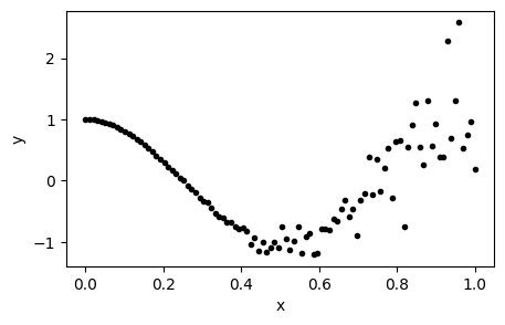
We’re going to train an approximate QEP on a 1D regression dataset with heteroskedastic noise.

# Define some training data
train_x = torch.linspace(0, 1, 100)
train_y = torch.cos(train_x * 2 * math.pi) + torch.randn(100).mul(train_x.pow(3) * 1.)

fig, ax = plt.subplots(1, 1, figsize=(5, 3))
ax.scatter(train_x, train_y, c='k', marker='.', label="Data")
ax.set(xlabel="x", ylabel="y")

[Text(0.5, 0, 'x'), Text(0, 0.5, 'y')]

Here’s a simple approximate QEP model, and a script to optimize/test the model with different objective functions:

POWER = 1.0
class ApproximateQEPModel(qpytorch.models.ApproximateQEP):
    def __init__(self, inducing_points):
        self.power = torch.tensor(POWER)
        variational_distribution = qpytorch.variational.CholeskyVariationalDistribution(inducing_points.size(-1), power=self.power)
        variational_strategy = qpytorch.variational.VariationalStrategy(
            self, inducing_points, variational_distribution, learn_inducing_locations=True
        )
        super().__init__(variational_strategy)
        self.mean_module = qpytorch.means.ConstantMean()
        self.covar_module = qpytorch.kernels.ScaleKernel(qpytorch.kernels.RBFKernel())

    def forward(self, x):
        mean_x = self.mean_module(x)
        covar_x = self.covar_module(x)
        return qpytorch.distributions.MultivariateQExponential(mean_x, covar_x, power=self.power)

# this is for running the notebook in our testing framework
import os
smoke_test = ('CI' in os.environ)
training_iterations = 2 if smoke_test else 200


# Our testing script takes in a QPyTorch MLL (objective function) class
# and then trains/tests an approximate QEP with it on the supplied dataset

def train_and_test_approximate_qep(objective_function_cls):
    model = ApproximateQEPModel(torch.linspace(0, 1, 100))
    likelihood = qpytorch.likelihoods.QExponentialLikelihood(power=model.power)
    objective_function = objective_function_cls(likelihood, model, num_data=train_y.numel())
    optimizer = torch.optim.Adam(list(model.parameters()) + list(likelihood.parameters()), lr=0.1)

    # Train
    model.train()
    likelihood.train()
    for _ in range(training_iterations):
        output = model(train_x)
        loss = -objective_function(output, train_y)
        loss.backward()
        optimizer.step()
        optimizer.zero_grad()

    # Test
    model.eval()
    likelihood.eval()
    with torch.no_grad():
        f_dist = model(train_x)
        mean = f_dist.mean
        f_lower, f_upper = f_dist.confidence_region()
        y_dist = likelihood(f_dist)
        y_lower, y_upper = y_dist.confidence_region()

    # Plot model
    fig, ax = plt.subplots(1, 1, figsize=(5, 3))
    line, = ax.plot(train_x, mean, "blue")
    ax.fill_between(train_x, f_lower, f_upper, color=line.get_color(), alpha=0.3, label="q(f)")
    ax.fill_between(train_x, y_lower, y_upper, color=line.get_color(), alpha=0.1, label="p(y)")
    ax.scatter(train_x, train_y, c='k', marker='.', label="Data")
    ax.legend(loc="best")
    ax.set(xlabel="x", ylabel="y")

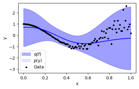
Objective Funtion 1) The Variational ELBO

The variational evidence lower bound - or ELBO - is the most common objective function. It can be derived as an lower bound on the likelihood \(p(\mathbf y \! \mid \! \mathbf X)\):

\[\mathcal{L}_\text{ELBO} = \sum_{i=1}^N \mathbb{E}_{q( \mathbf u)} \left[ \mathbb{E}_{f( \mathbf f \mid \mathbf u)} \left[ \log p( y_i \! \mid \! f_i) \right] \right] - \beta \: \text{KL} \left[ q( \mathbf u) \Vert p( \mathbf u) \right]\]

where \(N\) is the number of datapoints and \(p(\mathbf u)\) is the prior distribution for the inducing function values. For more information on this derivation, see Hensman et al., 2015.

How to use the variational ELBO in QPyTorch

In QPyTorch, this objective function is available as qpytorch.mlls.VariationalELBO.

train_and_test_approximate_qep(qpytorch.mlls.VariationalELBO)

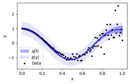
Objective Funtion 2) The Predictive Log Likelihood

The predictive log likelihood is an alternative to the variational ELBO that was proposed in Jankowiak et al., 2020. It typically produces predictive variances than the qpytorch.mlls.VariationalELBO objective.

\[\begin{split}\begin{align} \mathcal{L}_\text{PLL} &= \mathbb{E}_{p_\text{data}( y, \mathbf x )} \left[ \log p( y \! \mid \! \mathbf x) \right] - \beta \: \text{KL} \left[ q( \mathbf u) \Vert p( \mathbf u) \right] \\ &\approx \sum_{i=1}^N \log \mathbb{E}_{q(\mathbf u)} \left[ \int p( y_i \! \mid \! f_i) p(f_i \! \mid \! \mathbf u) \: d f_i \right] - \beta \: \text{KL} \left[ q( \mathbf u) \Vert p( \mathbf u) \right] \end{align}\end{split}\]

Note that this objective is very similar to the variational ELBO. The only difference is that the \(\log\) occurs outside the expectation \(\mathbb E_{q(\mathbf u)}\). This difference results in very different predictive performance.

How to use the predictive log likelihood in QPyTorch

In QPyTorch, this objective function is available as qpytorch.mlls.PredictiveLogLikelihood.

train_and_test_approximate_qep(qpytorch.mlls.PredictiveLogLikelihood)